Truncated determinants and the refined enumeration of Alternating Sign Matrices and Descending Plane Partitions (Algebraic Combinatorics related to Young diagram and statistical physics)

Truncated

determinants and the refined enumeration of

Alternating

Sign

Matrices and

Descending

Plane

Partitions

Philippe

Di Francesco

Institut

de Physique

Th\’eorique,

Commissariat

\‘a

l’Energie

Atomique,

Saclay, France

1

Introduction

Inthesenotes,

we

willbemainlyfocussing

on

the proofof the so-calledASM-DPP

conjec-tureofMills, Robbins andRumsey [22] which relates refinedenumerations ofAlternating

Sign Matrices (ASM) and DescendingPlane Partitions (DPP).

ASMs were introduced by Mills, Robbins and Rumsey [24] in their studyofDodgsons

condensation algorithm for the evaluation of determinants. DPPs were introduced by

Andrews [1] whileattemptingto prove

a

conjecturedformula for the generatingfunction

ofcyclically symmetric plane partitions.

1.1 ASMs from lambda-determinant

$Th-\bigcap_{ノ}$ definition of theso-called lambda-determinant ofMills, Robbins and Rumsey [24] is

based on the famous Dodgson condensation algorithm [12] for computing determinants,

itself based

on

theDesnanot-Jacobiequation,

a

particularPl\"uckerrelation,relating minors

of any square $k+1\cross k+1$ _matrix $M$:

$|M|\cross|M_{1,k+1}^{1,k+1}|=|M_{k+1}^{k+1}|\cross|M_{1}^{1}|-|M_{1}^{k+1}|\cross|M_{k+1}^{1}|$ (1.1)

where $|M_{\dot{|}12,1,}^{j_{1},j_{2}.’.\cdot\cdot.\cdot,j_{r}}|$ stands forthe determinant ofthematrixobtained from$M$ by deleting rows$i_{1},$ $i_{r}$ andcolumns$j_{1},$ $j_{f}$. The relation (1.1) maybeused

as

arecursion relation

on

thesize ofthe matrix, allowing for efficiently compute its determinant.

More formally,

we

may recast the algorithm using the so-called $A_{\infty}$ $T$-system (also

known

as

discrete Hirota) relation:

$T_{i,j,k+1}T_{i,j,k-1}=T_{j+1},{}_{ki,j-1,k}T-T_{i+1,j},{}_{ki-1,j,k}T$ (1.2)

for any $i,j,$$k\in \mathbb{Z}$ with fixedparity of $i+j+k$

.

Nowlet $A=(a_{i,j})_{i,j\in\{1,2,\ldots,n\}}$ be a fixed $n\cross n$ matrix. Together withthe initial data:

$T_{\ell,m,0}$ $=$ $1$ _{$(\ell, m\in \mathbb{Z};\ell+m=n mod 2)$} $T_{l,j,1}$

thesolution ofthe $T$-system (1.2) satisfies:

$T_{0,0,n}=\det(A)$ (1.4)

Given a fixed formal parameter $\lambda$, thelambda-determinant ofthe

matrix $A$, denoted

by $|A|_{\lambda}$ is simply defined

as

thesolution _{$T_{0,0,n}=|A|_{\lambda}$} of thedeformed $T$-system

$\tau_{i,j,k+1}T_{j,k-1}=T_{j+1,k}T_{j-1,k}+\lambda T_{i+1,j,k}T_{-1,j,k}$ (1.5)

subject to the initialcondition (1.3).

The discovery of Mills, Robbins and Rumsey is that the lambda-determinant is a

homogeneousLaurentpolynomial of the matrix entries of degree$n$, and that

moreover

the

monomials in the expression are coded by$n\cross n$ matrices $B$ withentries$b_{i,j}\in\{0, 1, -1\},$

characterized by the fact that their

row

andcolumn

sums are

1 and that the partial

row

andcolumnsums

are

non-negative, namely

$\sum_{i=1}^{k}b_{i,j}\geq 0 \sum_{i=1}^{k}b_{j,i}\geq 0 (k=1,2, n-1;j=1,2, \ldots, n)$

$\sum_{i=1}^{n}b_{i,j}=1 \sum_{i=1}^{n}b_{j,i}=1 (j=1,2, \ldots, n)$

Such matrices $B$ are called alternating sign matrices (ASMs). These include the

permu-tationmatrices (theASMs with no $-1$ entry). Here

are

the 7 ASMsof size 3:

$(\begin{array}{lll}1 0 00 1 00 0 1\end{array})(\begin{array}{lll}1 0 00 0 10 l 0\end{array})(\begin{array}{lll}0 1 01 0 00 0 1\end{array})(\begin{array}{lll}0 1 0l- 1 101 0\end{array})(\begin{array}{lll}0 1 00 0 11 0 0\end{array})(\begin{array}{lll}0 0 11 0 o0 1 0\end{array})(\begin{array}{lll}0 0 10 1 o1 0 0\end{array})$

Thereis an explicit formula for thelambda-determinant[24]:

$|A|_{\lambda}= \sum_{n\cross nASMB}\lambda^{Inv(B)-N(B)}(1+\lambda)^{N(B)}\prod_{i,j}a_{i,j^{j}}^{b}$ (1.6)

where $Inv(B)$ and $N(B)$ _{denote respectively the inversion number and the number of}

entries $-1$ in $B$, with

$Inv(B) = \sum_{1\leq k<\ell\leq n1\leq i<j\leq n} b_{i,\ell}b_{j,k}$

$N(B) = \frac{1}{2}(-n+\sum_{1\leq i,j\leq n}|b_{i,j}|)$

Note that for $\lambda=-1$, only the

ASMs

_{with $N(B)=0$ contribute, i.e. the permutation}

matrices, for which$Inv(B)$ _{coincideswith the usual inversion numberof thecorresponding}

permutation, and therefore (1.6) reduces to the usual formula for the determinant.

Mills, Robbins and Rumsey [22] noticed that apart from the quantities $Inv(B)$ _and

any

ASM.

We denote by $t(B)$ the number of$0$

entries

to the left of the

1

in the top

row

of $B.$

Associating aweight

$W(B)=z^{t(B)}y^{Inv(B)-N(B)_{X}N(B)}$ _(1.7)

to each ASM $B$, wemay form the partitionfunction

$Z_{ASM}^{(n)}(x, y, z)= \sum_{n\cross nASMB}W(B)$ (1.8)

In thecase$n=3$listedabove,theASMsreceive respective weights: 1,$zy,$$zxy,$$y,$$zy^{2},$$z^{2}y^{2},$ $z^{2}y^{3},$

leading to $Z_{ASM}^{(3)}(x, y, z)=1+zy+zxy+y+zy^{2}+z^{2}y^{2}+z^{2}y^{3}.$

1.2 DPPs

Descending plane partitions

are

arrays ofpositive integers of the form:

$a_{1,1}$ $a_{1,2}$ $a_{1,3}$

. . .

.. .

$a_{1,\mu_{1}-2}$ $a_{1,\mu_{1}-1}$ $a_{1,\mu_{1}}$ $a_{2,2}$ $a_{2,3}$

.

.

.

$\cdots$

$a_{2,\mu_{2}}$ $a_{3,3}$

. . .

$a_{3,\mu_{3}}$

$\cdots$

$a_{r,r}\cdots a_{r,\mu_{r}}$

such that the sequece $\mu_{i}$ is strictly decreasing $\mu_{i+1}<\mu_{i}$, and that for $\lambda_{i}=\mu_{i}-i+1,$

$\lambda_{0}=\infty$:

$a_{i,j}\geq a_{i,j+1} a_{\iota,j}>a_{i+1,j} \lambda_{i}<a_{i,i}\leq\lambda_{i-1}$

for all$i,$$j$. By convention, the empty partition is aDPP. Here

are

the7 DPPs oforder 3:

3 3

$\emptyset, 2, 3, 3 1, 3 2, 3 3,$

2

The integers $a_{i,j}$ are called parts. A DPP $A$ is said to be of order $n$ if $a_{i,j}\leq n$ for

all $i,$ $j$. A part $a_{i,j}$ is said to be special if$a_{i,j}\leq j-i$. We denote by $S(A)$ and $NS(A)$

respectivelythe total number of specialpartsand thetotalnumber of non-specialpartsof

any DPP $A$

.

Another observable ofinterest among theDPPs $A$ of order $n$is thenumber

of parts in $A$ equal to the order, which

we

denote by _$M(A)$

.

To each DPP $A$ of given

order, we associate aweight

$W(A)=x^{S(A)}y^{NS(A)_{Z}M(A)}$ _(1.9)

and define thepartition function for DPPs of order $n$to be:

$Z_{DPP}^{(n)}(x, y, z)= \sum_{DPPA\circ fordern}W(A)$ (1.10)

The7DPPsof order3listedabovehave respective weights: 1,$y,$$zy,$$zxy,$$zy^{2},$$z^{2}y^{2},$$z^{2}y^{3},$

as $M(A)$ _{isthenumberof}

occurrences

_{ofthe part 3, and the only special partis the entry}

1 in thefourth DPP. This leads to the partitionfunction$Z_{DPP}^{(3)}=1+y+zy+zxy+zy^{2}+$

1.3 The ASM-DPP conjecture

The ASM-DPP conjecture

as

stated byMills, Robbins and Rumsey [22] amounts to the

identity between the partition functions of ASMs and DPPs

as

defined in the previous

sections. This isthe following:

Theorem 1.1. Thepartition

_{functions for}

the

_refined

enumeration

_of

ASMs and DPPs

coincide, namely

$Z_{ASM}(x, y, z)=Z_{DPP}(x, y, z)$

This wasfinally proved in all its generality in [4], and then generalized so

as

to include

yet another observable in [5]. In the present note,

we

explain the rationale behind these

proofs whichstrongly rely onmanipulations offinitetruncations of infinite matrices.

For simplicityofexpositionwe shall start withthe identitybetween the doublyrefined

partition functions $Z_{ASM}^{(n)}(x, y, 1)$ _and $Z_{DPP}^{(n)}(x, y, 1)$

.

Each will be expressed

as

the

deter-minantofafinite truncation (of size$n\cross n$) ofan infinitematrix, and theidentitybetween

determinants will bederived from general principles relating the two $\langle$

infinite” matrices.

One key ingredient is the

use

ofthe double generating series for the matrix entries (see

Appendix A for definitions and properties).

1.4 Outline

The use of infinite matrices is somewhat non-standard in this context, andwe would like

tostress the power and beauty of the method. The infinite matrices occurring here

actu-ally involve

some

fundamental object that

came

up in the study of so-called Lorentzian

triangulations [8], giving rise to

one

of the simplest examples ofquantumintegrable

sys-tem. More precisely, random configurations ofthis particularclass oftriangulations may

be generated by iterated powers ofa transfer matrix$T$ ofinfinite size. The problemwas

solved exactly by diagonalization of $T$ in [8]. A drastic simplification of the problem

comesfrom the existence ofaninfinite parametricfamily of such transfermatrices, which

all commute with each other.

The notes areorganized as follows.

InSection 2,

we

recallanumberoffacts about the transfermatrixof$1+1$-dimensional

Lorentzian triangulations, including other applicationstotrees and lattice path

enumer-ation.

In Section 3,

we

compute $Z_{ASM}^{(n)}(x, y, 1)$ by

use

of the Izergin-Korepin (IK) [15, 17]

determinant formulation of the partitionfunction of the bijectively equivalent

configura-tions ofthe 6Vertex (6V) modelwith Domain-WallBoundaryConditions (DWBC). The

difficulty here is to extract a homogeneous hmit out ofthe IK determinant, and to put

it in theform ofthe determinant of a finite truncation to size $n\cross n$ ofan infinite matrix

which is independent of$n.$

In Section 4, we compute $Z_{DPP}^{(n)}(x, y, 1)$ _by use of the lattice path formulation of the

problem [19], and by use of the Lindstr\"om Gessel-Viennot (LGV) determinant formula for the partition function of non-intersecting families of lattice paths. This expresses

$Z_{DPP}^{(n)}(x, y, 1)$

as

_{thedeterminant}of_thefinite_{truncation to size} $n\cross n$ofan infinite matrix

InSection 5,

we

show how the relation between the double generating

functions

of the

two infinite matrices above implies the identity between the determinants of any finite

truncation thereof. This is the key to the proof of the ASM-DPP conjecture. We then

show how this hasto be adapted to include more refinements.

In theconclusive Section6, theASM-DPP correspondence is placed in thewider

con-text ofthe myriadof combinatorialobjects and physical systemsconnectedto ASMs. We

alsocompare the twovery different forms ofquantum integrability underlying the

ASM-DPP correspondence,

one

coming fromthe Lorentzian triangulations, the other from the

$6V$model.

We collect the useful formulas and definitions for generatingfunctions and truncated

determinants of infinite matrices in Appendix A.

Acknowledgments. These notes

are

largely based

on

work with E. Guitter,

C.

Krist-jansen, R. Behrend and P. Zinn-Justin. I thank the Mathematical Sciences Research

Instiitute, Berkeley, California for hosting

me

while thesenotes

were

completed.

2

The

main actor: the transfer matrix of Lorentzian gravity

2.1 $1+1D$ Lorentzian gravity

Discrete models for $1+1D$ Lorentzian gravity are defined

as

_{follows. They}

are

_statistical

models whose configurations

are

discretespace-times,in the formofrandom triangulations

witharegular discrete timedirection $(an$integersegment $[t_{1}, t_{2}]\subset \mathbb{N})$ and

a

randomspace

direction, modeled by random triangulations of the unit time strips $[t, t+1],$ $t\in \mathbb{N}$, by

arbitrary but finitenumbers oftriangles with

one

edge along the time line $t$ (resp. _$t+1$)

and the opposite vertex

on

the time line $t+1$ _(resp. $t$). All other edges

are

thenglued

to their neighbors

so

as

to formatriangulation. Each “horizontaledge”’ along

a

time line

$t$ is shared by two triangles,

one

in each timeslice $[t-1, t]$ and _$t,$$t+1$]. The boundary

conditions alongthe time lines may be taken free, periodicor staircase-like [8]. A typical

free boundary Lorentzian triangulation $\Theta$ in _$1+1D$reads

as

follows:

space

Thesetriangulations

are

best described in the dualpicture by considering triangles

as

vertical half-edges andpairsof trianglesthat shareatimelike (horizontal) edge

as

vertical

between two consecutive time-slices which typically reads

as

follows:

(2.1)

with say $i$ half-edges on the bottom and $j$ on the top (here for instance

we

have $i=9$

and$j=10)$

.

Denoting by $|i\rangle$ and $|j\rangle$,

withl

$i,j\in \mathbb{Z}_{+}$, the bottom and top Hilbert space

statebases,

we

may describe thegenerationof

a

triangulation bythe iterated action of a

transferoperator7withmatrix elements$T_{i,j}=(\begin{array}{l}i+ji\end{array})$ betweenstates $|i\rangle$ and $|j\rangle$

.

Note that

the corresponding matrix $T=(T_{i,j})_{i,j\in z_{+}}$ is infinite. We shall deal with such matrices

in the following. As detailed in Appendix $A$,

a

compact characterization of the infinite

matrix$T$ isviaits double generating function:

$f_{T}(u, v)= \sum_{i,j\geq 0}T_{i,j}u^{i_{l)}j}=\frac{1}{1-u-v}.$

2.2 Integrability

To make the model more realistic, we may include both area and curvature-dependent

terms, by introducing Botlzmann weights $w(\Theta)$ equal to the product of local weights of

theform $g$per triangle (area term) and $a$per pair ofconsecutive triangles in

a

time-slice

pointing in the

same

direction, either both up

or

both down (curvature term). The rules

in the dual picture are as follows:

$T \perp T \perp$

$g$ $g$

a

a

For instance, in the example (2.1) above with $i=9$ and $j=10$ , the product of local

weights is $g^{19}a^{9}$

.

For the staircase-like boundaryconditions of [8], namely assuming that

eachstate-to-state transition

as

in (2.1) hasat leastone leftmosthalf-edgeonthe bottom

andonerightmosthalf-edgeontop (andnot counting theleftmost and rightmost half-edge

weights $g^{2}$), it is easy tocomputethe new transfer operator$T(g, a)$ withmatrix elements

$\tau(9^{a})_{i,j}=(ag)^{i+j}\sum_{k=0}^{{\rm Min}(iij)}(\begin{array}{l}ik\end{array})(\begin{array}{l}jk\end{array})a^{-2k}$ (2.2)

for$i,$$j\geq 0$which expressesthe transitionbetween states $|i+1\rangle$ and $|j+1\rangle$

.

Equivalently,

the double generatingfunctionreads:

$f_{T(g_{)}a)}(u, v)= \sum_{i,j\geq 0}T(g, a)_{i,j}u^{i}v^{j}=\frac{1}{1-ga(u+v)-g^{2}(1-a^{2})uv}$ (2.3)

and

we

have$T(g, a)=T(ga, ga, g^{2}(1-a^{2}))$ in thenotations of Appendix A.

This model turns out to provide

one

of the simplest examples ofquantum integrable

system, with

an

infinite family ofcommuting transfer matrices. Indeed,

we

have:

Theorem 2.1. [8] The

_transfer

matrices$T(g, a)$ _and$T(g’, a’)$ _commute

_if

_{and only}

_if

_the

parameters$(g, a, g’, a’)$

are

_{such that}$\varphi(g, a)=\varphi(9’, a’)$ where:

$\varphi(g, a)=\frac{1-g^{2}(1-a^{2})}{ag}$ (2.4)

This is easily proved by using the generating functions. This case corresponds to the

familyofmatrices $T_{s,t}(\alpha)$ of Appendix $A$, with _$s=1,$ $t=\varphi(g, a)$ and $\alpha=ga.$

2.3 Diagonalization

To diagonalize $T$, we may first consider finite size truncations _{$T^{[0,k]}=(T_{i,j}(g, a))_{i,j\in[0,k]}.$}

It is easy to

see

thatthe $(k+1)\cross(k+1)$ symmetric matrix $T^{[0,k]}$ _{is diagonalizable, with}

eigenvalues $\lambda_{i}^{[0,k]}(g, a)=g^{2i}(1+O(g^{2}))$_, $i\in[0, k]$_{, all with formal series expansions in}

powers of$g$ with coefficients in $\mathbb{Z}[a]$

. As

$k$ increases, we get

more

and

more

eigenvalues,

with powerseries expansions that stabilize. Inthissense, thehmiting infinitematrix has

an

infinite set ofeigenvalues $\lambda_{i}=g^{2i}(1+O(g^{2}))$, $i\in \mathbb{Z}_{+}$, with well-defined formal power

series expansions in $g.$

Setting $\varphi(g, a)=q+q^{-1}$ for

some

$q\in \mathbb{C}^{*}$, and introducing

a

newvariable

$\lambda=\frac{1-q^{-1}ga}{1-qga},$

we

may rewrite the double generating function of$\tau(9^{a})$

as:

$f_{T(g,a)}(u, v) = \frac{1-\lambda q^{2}}{(1-qu)(1-qv)-\lambda(u-q)(v-q)}$

$= \sum_{m=0}^{\infty}\frac{\sqrt{1-q^{2}}(q-u)^{m}}{(1-qu)^{m+1}}(\frac{1-\lambda q^{2}}{1-q^{2}}\lambda^{m})\frac{\sqrt{1-q^{2}}(q-v)^{m}}{(1-qv)^{m+1}}$ (2.5)

where

we

identify

$\Lambda^{(m)}=\frac{1-\lambda q^{2}}{1-q^{2}}\lambda^{m}$

as

the m-th eigenvalue of$T(g, a)$, $m\in \mathbb{Z}_{+}$ and

$f_{v^{(m)}(u)}= \sum_{i=0}^{\infty}v_{i}^{(m)}u^{i}=\frac{\sqrt{1-q^{2}}(q-u)^{m}}{(1-qu)^{m+1}}$

as

the generating function for thecorresponding eigenvector $v^{(m)}$

.

Note that $(v^{(m)})_{m\in Z_{+}}$

forman orthonormalbasisof the Hilbertspaceof states w.r.$t$

.

thestandardscalar product

$u \cdot v=\sum_{i\in Z_{+}}u_{t}v_{i}$. It is easy to show that$\Lambda^{(m)}=g^{2m}(1+O(g^{2}))$

as

a formalpowerseries of$g$, thereby proving that theseare thelimits of the eigenvaluesofthetruncatedmatrices

as

the size $karrow\infty.$

This

was

extensivelyused in [8] to compute correlationfunctions oftop/bottom

bound-ary loops in random Lorentzian triangulations. We want to stress here the very simple

2.4 Trees

For staircase boundary conditions, the dual random Lorentzian triangulations introduced

above may be viewed

as

random plane trees. This is easily realized by gluing all the

bottom vertices ofparallel vertical edges whose both top and bottom halves contribute

to the curvature term (no interlacing with the neighboring time slices). A typical such

example reads:

Note that the tree is naturally rooted at its bottom vertex.

To summarize, we have unearthed

some

integrable structure abtached naturally to

certain plane trees. Note that intree language the weights are respectively $g^{2}$ per edge

(except the left/right boundaryones), and$a$perpairof consecutive descendent half-edges

(fromleft to right) and per leaf.

2.5 Paths

There is yet another interpretation of the transfer matrix $T(g, a)$ _of $1+1D$ Lorentzian

gravity, in terms of lattice paths. First notice that $T(g, a)=V(g, a)V^{t}(g, a)$ _for

_some

(infinite) lowertriangular matrix $V(g, a)$ with entries

$V(g, a)_{i,k}=g^{i}a^{i-k}(\begin{array}{l}ik\end{array}) (i, k\in \mathbb{Z}_{+})$ (2.6)

and double generating function:

$f_{V(g,a)}(u, v)= \frac{1}{1-agu-guv}$ (2.7)

In the notationsofAppendix A.2, we have $V(g, a)=L(a^{-1}, ga)$

.

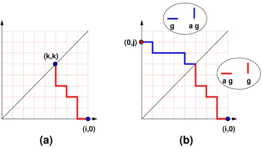
Consider paths

on

the positive quadrant of the two-dimensional square lattice $\mathbb{Z}+^{2},$

with steps $(-1, O)$ _{(horizontal) and} $(0,1)$ (vertical),

as

illustrated in Fig.$1(a)$

.

Then the

total number of paths from the point $(i, 0)$ to the point $(k, k)$

on

the diagonal is $(\begin{array}{l}ik\end{array}).$

Moreover ifwe attach a weight $ga$ per horizontal step and $g$ per vertical one, we get

a

total contribution of$(ga)^{k-i}g^{k}(\begin{array}{l}ik\end{array})=V(g, a)_{i,k}$, whichweinterpretasthepartition function

for weightedpaths from $(i, 0)$ to $(k, k)$. This quantity will also reappear later.

Note that in this language$T(g, a)_{i,j}$isthepartitionfunctionof lattice paths from$(i, 0)$

to $(0,j)$ _{in the positive quadrant, with weights} $9^{a}$ (resp. g) per horizontal step below

(resp. above) the diagonal and $g$ (resp. $ga$) per step above (resp. below) the diagonal

(i,O)

$($

a

$)$

$(i,0)$

$($

b

$)$

Figure 1: A typicalpath contributingto the matrix element$V(g,a):,k(a)$, and to$T(g,a):,j(b)$.Thesepathsare

taken on$\mathbb{Z}_{+}^{2}$, with steps$(-1,0)$and _$(0,1)$. Inthe lattercase, wehaveindicatedtheweights ofthe steps below

and above thediagonal.

Thisformulation allowstovisualizeimmediately thetruncatedtransfermatrix$T^{[0,k]}(g, a)$

as

corresponding to paths within the square $[0, k]\cross[0, k]\subset \mathbb{Z}_{+}^{2}$

.

For such paths, both

the portion below the diagonal and that above

are

within the

same

square,

so

that

we

may write $T^{[0,k]}(g, a)=V^{[0,k]}(g, a)V^{[0,k]}(g, a)^{t}$, wich immediately yields the determinant

of$T^{[0,k]}$,

as

$V^{[0,k]}(g, a)$ is lower triangular (see also Appendix A.4):

$\det(T^{[0,k]}(g, a))=\det(V^{[0,k]}(g, a))^{2}=g^{k(k+1)}$

This iscompatible witheigenvalues $\lambda_{i}^{[0,k]}(g, a)=g^{2_{l}}(1+O(g^{2}))$ _{for $i=0$}, 1, $k.$

3

Enumerating

ASMs

3.1 ASMs, $6V$ model and the IK deteminant

As discovered by Kuperberg [18], ASMs of size $n\cross n$

are

in bijection with the so-called

Domain-Wall Boundary Condition Six Vertex ($6V$-DWBC) model

on a

square grid of size

$n\cross n$

.

The latter configurations

are

choices oforientations of the edges of

a

$n\cross n$ grid

of the $(tw(\succ$dimensional) square lattice, in such a way that at each vertex exactly two

edges point $tx$ and two point from- the vertex. Moreover oriented external horizontal

(resp. vertical) edges

are

attached to the boundary vertices, in sucha way that external

horizontal edgespointtowards thegrid and verticalonesfrom the grid. Wedisplay below

the6 possible vertex configurations $a_{1},$$a_{2},$$b_{1},$$b_{2},$

a sample grid showingthe external edge boundary condition:

We have also indicated the dictionary between the vertex configurations and the ASM

entries. It is easy to understand the bijection as follows. The $\pm 1$ entries correspond

to vertices where both the horizontal and vertical flows (indicated by the direction of

the edges) are

_reflected.

The alternation of 1 and $-1$ _entries corresponds to odd _and

even order flips along each row or column ofthe grid. The DWBC boundary condition

ensures

that thefirst and last encountered

non-zero

elements in theASM along

rows

and

columns must be 1,

as

one needs

an

odd total number offlips to

reverse

the external edge

orientation, when goingalonga row or a column.

The$6V$ modelhad been extensively studied in the physics literature. With a _suitable

parameterization of the Boltzmann weights $a_{i},$$b_{i},$$c_{\tau}$, the model forms the archetypical

example of

an

integrable lattice model, as it admits an infinite family of commuting

transfer matrices, that

can

be diagonalized for various types of bopundary conditions

usingthe Bethe Ansatztechniques. Theseintegrableweights aredefined

as

follows. Each

row (resp. column) of the grid carries a complex number $z_{i},$ $i=1$,2, $n$ (resp. $w_{i},$

$i=1$,2, n $)$ called spectral parameter. Moreover the weights depend on a “quantum

parameter$q\in \mathbb{C}^{*}$

.

We havethe following parametrizationofthe weights:

$a(z, w)=qz-q^{-1}w b(z, w)=q^{-1}z-qw c(z, w)=(q^{2}-q^{-2})\sqrt{zw}$

where $a(z, w)$ _{is the}weight fora vertex oftype $a_{1}$ or$a_{2}$ at the intersectionof aline with

parameter $z$ and column with parameter $w$, etc. With this parameterization, the model

has an infinite family of commuting row-to-row transfer matrices, and

can

be exactly

solved by BetheAnsatz techniques. Using recursion relationsofKorepin [17], Izergin [15]

obtained a compact determinantal formula for the partition function of this $6V$-DWBC

model, definedasthe sum

over

edge configurations of theproductof local vertex weights,

divided by thenormalizationfactor $\prod_{i=1}^{n}c(z_{i}, w_{i})$ (tomake the

answer

polynomial in the

$z$’sand $w’ s$). It reads:

$Z_{6V}^{(n)}(q; \{z_{i}\}, \{w_{j}\})=\frac{\prod_{i,j}a(z_{i},w_{j})b(z_{i},w_{j})}{\Delta(z)\triangle(w)}det1\leq i,j\leq n(\frac{1}{a(z_{i},w_{j})b(z_{i},w_{j})})$ (3.1)

where $\triangle(z)=\prod_{1\leq i<j\leq n}(z_{i}-z_{j})$ stands for the Vandermonde determinant ofthe $z’ s.$

3.2 Homogeneous limit and computation of$Z_{ASM}^{(n)}(x, y, 1)$

In the above bijection between $6V$ configurations _{and ASMs, it is} easy to track both

quantities $N(B)$ _and$Inv(B)$ in terms of$6V$weights. We find that

where$N_{a}.,$ $N_{b}.,$ $N_{c_{1}}$ stand for the total numbers of vertex configurations of eachtype. The

determinant result above

can

therefore be usedto compute the refined partition function

$Z_{ASM}^{(n)}(x, y, 1)$forASMs, whichcounts ASMs with aweight$x/y$perentry $-1$ and

a

weight

$y$ for eachinversion. Setting

$x=( \frac{c}{b})^{2} y=(\frac{a}{b})^{2}$ (3.2)

we

have:

$Z_{ASM}^{(n)}(x, y, 1)= \sum_{ASMB}x^{N(B)}y^{Inv(B)-N(b)}=b^{-n(n-1)}Z_{6V}^{(n)}(a, b, c)$ (3.3)

where$Z_{6V}^{(n)}(a, b, c)$ referstothehomogeneous limit of thepartitionfunction (3.1) of the$6V$

model in which all$a(z_{i}, w_{j})$ tend to$a$, etc. This is obtained by letting all $z_{1}arrow r$ and all

$w_{i}arrow r^{-1}$, with $a=a(r, r^{-1})$, $b=b(r, r^{-1})$ _and $c=c(r, r^{-1})$. This and more refinements

were

worked out in [4]. We have the followingremarkable result:

Theorem 3.1. [4] The partition

_{function for refined}

ASMs reads:

$Z_{ASM}^{(n)}(x, y, 1)=0\leq i_{1}j\leq n-1\det((1-\nu)I+\nu G)$ (3.4)

where $\nu$ is any solution to the equation

$x\nu(1-\nu)=\nu+y(1-\nu)$ (3.5)

and the$n\cross n$ determinant is the principal minor

for

the $n$

first

rows

and columns

of

the

infinite

matrix$M_{ASM}=(1-\nu)I+vG$ whose entries

are

generated by

$f_{M_{ASM}}(u, v)= \frac{1-\nu}{1-uv}+\frac{\nu}{1-xu-v-(y-x)uv}$ (3.6)

Note theremarkablesimilarity between the generatingfunction for thematrix elements

of$G$ and the that of the transfer matrix for $1+1D$ Lorentzian triangulations (2.3). The

two actually match up to

a

rescaling $uarrow u/\sqrt{x}$ and $varrow v\sqrt{x}$ (which amounts to

a

conjugation by the diagonal matrix $\sqrt{x}I$) and upon identifying $x=g^{2}a^{2}$ and $y=g^{2}.$

Note also that $G=T(x, 1, y-x)$ in thenotations ofAppendix A.2.

Let

us

now

give

a

sketch of the proof of Theorem 3.1. The determinant (3.1) is

singular in the homogeneous limit, but we may Taylor-expand the matrix entries within

the determinant around the homogeneous point. For $a=a(r, r^{-1})$, $b=b(r, r^{-1})$ _and

$c=c(r, r^{-1})$ _{this reads:}

$Z_{6V}^{(n)}(a, b, c)= \frac{(ab)^{n^{2}}}{c^{n}}\det 0\leq i,j\leq n-1(\{(\frac{1}{i!}\frac{\dot{\theta}}{du})(\frac{1}{j!}\frac{d^{j}}{dv^{j}})\frac{c(u^{-1},v)}{a(u^{-1},v)b(u^{-1},v)}\}|_{u=v=r^{-1}})$

Noting further that

$\frac{c(u^{-1},v)}{a(u^{-1},v)b(u^{-1},v)}=\frac{1}{uv-q^{-2}}-\frac{1}{uv-q^{2}}$

and introducingthe infinite matrices $A_{\pm}$ with elements:

$(A_{\pm})_{i,j}= \{(\frac{1}{i!}\frac{d^{i}}{du^{i}})(\frac{1}{j!}\frac{d^{j}}{dv^{j}})\frac{1}{uv-q^{\pm 2}}\}|_{u=v=r^{-1}} (i,j\in \mathbb{Z}_{+})$ (3.7)

Lemma 3.2. We have

$A \pm=\frac{1}{r^{-2}-q^{\pm 2}}(U(\alpha_{\pm}, \beta_{\pm})^{t})^{-1}U(\alpha_{\pm}’,\beta_{\pm}’)$ (3.8)

for

$U(\alpha, \beta)$ the

infinite

upper triangular matrix with entries $U(\alpha, \beta)_{i,j}=(\begin{array}{l}ji\end{array})\alpha^{i}\beta^{j}$ (see

Appendix A.2), and where theparameters read:

$\alpha_{+}=\frac{1-q^{2}r^{2}}{r}, \beta_{+}=\frac{q^{2}-q^{-2}}{r^{2}-q^{2}},\alpha_{+}’=-q^{2}r^{2}\beta_{+}, \beta_{+}’=-\frac{1}{\alpha+}$

and the parameters with –index are obtained

_form

those with $+by$ the substitution

$qarrow(\Gamma^{1}.$

Proof.

The statement of the lemma is an immediate consequence ofthe fact that the

Taylor-expansionexpression (3.7) around $(u, v)=(r^{-1}, r^{-1})$ turnsinto the following

dou-blegenerating functions forthe matrix elements of$A_{\pm}$:

$f_{A\pm}(u, v)= \sum_{i,j\in Z_{+}}(A_{\pm})_{i,j}u^{i}v^{j}=\frac{1}{(r^{-1}+u)(r^{-1}+v)-q^{\pm 2}}$

Moreover, usingthe generatingfunction for the matrix elements of $U(\alpha, \beta)$ ofAppendix

A.2:

$f_{U(\alpha,\beta)}(u, v)= \frac{1}{1-\beta v(1+\alpha u)},$

andfor $\alpha\beta\neq 0,$ $U(\alpha, \beta)^{-1}=U(-1/\beta, -1/\alpha)$, wefinallycomputebyconvolution product: $f_{U^{t}(\alpha,\beta)^{-1}U(\alpha_{)}’\beta’)}(u, v) = f_{U(-1/\beta,-1/\alpha)}(v, u)*f_{U(\alpha’,\beta’)}(u, v)$

$= \oint_{C}\frac{dt}{2i\pi t}\frac{1}{1+\frac{1}{\alpha}u(1-\frac{1}{\beta}t^{-1})}\frac{1}{1-\beta^{J}v(1+\alpha^{J}t)}$

1

$= \overline{(1+\frac{1}{\alpha}u)(1-\beta^{J}v)-uv\frac{\alpha’\beta’}{\alpha\beta}}$

The lemmafollows from comparingthis with the expressions for $f_{A\pm}(u, v)$

.

$\square$

The Lemma is easily extended to finite truncations of the infinite matrices $A_{\pm}$ and

$U$,

as

$U$ is upper triangular and $(U^{t})^{-1}$ is lower triangular. Therefore

we

may write

$A_{\pm}^{[0,n-1]}= \frac{1}{r^{-2}-q^{\pm 2}}(U_{\pm}^{[0,n-1]t})^{-1}U_{\pm}^{[0,n-1]’}$withthe obviousshorthandnotations. Goingback

to our original determinant, we find that

$Z_{6V}^{(n)}(a, b, c)= \frac{(ab)^{n^{2}}}{c^{n}}\det(A_{-}^{[0,n-1]}-A_{+}^{[0,n-1]})$

$=$ $\frac{(ab)^{n^{2}}}{c^{n}}\det(A_{-}^{[0,n-1]})\det(\mathbb{I}-\frac{r^{-2}-q^{-2}}{r^{-2}-q^{2}}U_{-}^{[0,n-1]}t(U_{+}^{[0,n-1]t})^{-1}U_{+}^{[0,n-1]’}(U_{-}^{[0,n-1]’})^{-1})$

where $\mathbb{I}$

stands for the $n\cross n$ identity matrix. The last product of 4 matrices is finally

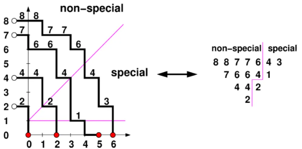
Figure2: Non-intersectinglatticepath configuration forasample DPPof order$n\geq 8$. _Wehaveindicatedthe

domains in which horizontal steps correspond to$special/non$-specialparts.

whereas the determinant of$A_{-}^{[0,n-1]}$ _{follows from its expression}

as

a_product oftriangular

matrices. Collectingall the factorsfinally yields (3.4-3.6),withthe followingidentification

ofparameters:

$x=( \frac{q^{2}-q^{-2}}{q^{-1}r-qr^{-1}})^{2}$ $y=( \frac{qr-q^{-1}r^{-1}}{q^{-1}r-qr^{-1}})^{2}$ $\nu=\frac{r^{-2}-q^{-2}}{q^{2}-q^{-2}},$ $1- \nu=\frac{q^{2}-r^{-2}}{q^{2}-q^{-2}}.$

4

Enumerating DPPs

4.1 Lattice path formulation ofDPPs

TheDPPs arein bijection with configurations ofnon-intersecting lattice paths illustrated

in Fig.2 and defined as follows. Like in Sect. 2.5, the paths take place in the positive

quadrant $(\mathbb{Z}_{+})^{2}$, with the samesteps but different weights and boundary conditions. The

paths start along the $x$ axis at positions ofthe form $(s_{i}, 0)(i=1,2,$ $r$ recorded from

right toleft) and end alongthe $y$axis at positions $(0, s_{i}+2)(i=1$, 2, $r$recorded from

top to bottom). We add

a

final horizontal left step at the end of each path. Reading

pathsfrom left toright andtoptobottom,

we

record the verticalpositions$y=a_{1,j}$ of the

j-th horizontalstep from the left taken

on

the i-th path from top (steps with $y=0$

are

not recorded). These form

a

DPP with $r$ rows, of order any $n\geq s_{1}+2$

.

Conversely to

eachDPP with$r$rows wemay associate such apath configuration. Note that the starting

points are such that $s_{i}=\lambda_{i}-1$, where $\lambda_{i}=\mu_{i}-i+1$ thetotal number of parts inthe

row $i.$

The special parts correspond to horizontal steps taken in the strict upper octant $y\geq$

$x+1$ of the plane, and the remaining parts correspond to the horizontal steps in the

4.2 Computation of$Z_{DPP}^{(n)(}(x, y, 1)$

Thecomputationof$Z_{DPP}^{(n)}(x, y, 1)$

uses

_theLindstr\"om-Gessel-Viennot _{[21, 14] determinant}

formula expressing the partition function for non-intersecting lattice paths with fixed

atarting points and endpoints $Z$

as

a determinant $\det(Z_{i,j})$ where $Z_{i,j}$ is the partition

function for asinglepathfrom the i-th starting point to the j-th endpoint. This leads to

the following:

Theorem 4.1. [4] Thepartition

_function

$Z_{DPP}^{(n)}(x, y)$

for

DPPs

of

order$n$ with weight$x$

per special part and$y$perotherpartreads:

$Z_{DPP}^{(n)}(x, y)=\det(\mathbb{I}+H^{[0,n-1]})$ _(4.1)

where the determinant is that

_of

the

_finite

truncation to the $n$

first

rows and columns

of

the

infinite

matrix$(M_{DPP})_{i,j}=\delta i,$$j+H_{i,j},$ $i,$$j\in \mathbb{Z}_{+}$, with generating

function:

$f_{M_{DPP}}(u, v)= \sum_{i,j\in Z+}(M_{DPP})_{i,j}u^{i}v^{j}=\frac{1}{1-uv}+\frac{1}{1-u}\frac{yu}{1-xu-v-(y-x)uv}$ (4.2)

Again, note the close similarity between the matrix $H$ and the transfer matrix $T$

for $1+1D$ Lorentzian triangulations. Our proof of the

ASM-DPP

conjecture will be

based on this similarity. Note also that in the notations of Appendix A.2, we have

$H=yS(\mathbb{I}-S)^{-1}T(x, 1, y-x)$

.

Let

us now

sketch the proofof Theorem 4.1. The sought after partition function is

a

sum

over all configurations of $r$ non-intersecting paths $(0\leq r\leq n-1)$ with fixed

$r$ starting points $(s_{i}, 0)$, $i=1,$ $r$ and endpoints $(0, s_{i}+2)$, $i=1,$ $r$

.

According

to the Lindstr\"om-Gessel-Viennot theorem, this is the sum over minors $|D|_{s_{1}^{1},\ldots,s_{r}^{\tau}}^{s,\ldots,s}$ of the $n\cross n$matrix$D$whose entries $D_{i,j}$ isthe partitionfunction fora single pathfrom $(i, 0)$ to

$(0,j+2)$

.

It also has thesimple expression:

$\sum_{r=0}^{n-1}\sum_{0\leq s_{1}<\ldots<s_{r}\leq n-1}|D|_{s_{1},\ldots,s_{r}^{r}}^{s_{1},\ldots,s}=\det(\mathbb{I}+D)$

Such a path is split into three pieces: (i) between the $x=0$ axis and the first hit on

the $x=1$ axis (ii) between the $x=1$ axis and the diagonal line $y=x+1$ (iii) between

the diagonal line $y=x+1$ and the vertical axis $y=$ O. Each piece receives a specific

weight, with total contribution:

$D_{i,j}= \sum_{k=0}^{i}\sum_{\ell=0}^{{\rm Min}(k,j+1)}(\begin{array}{l}k\ell\end{array})x^{k-\ell}(\begin{array}{ll}j +1 \ell\end{array})y^{\ell+1}$ (4.3)

where we have first summed over (i) paths from $(i, 0)to(k, 1)$ with $i-k$ horizontalsteps

along the $x=0$ axis and one final vertical step (ii) paths from $(k, 1)$ to $(\ell, \ell+1)$ on the

diagonal $y=x+1$, for which $k-\ell$ horizontal _steps must be chosen among a _total of

$k$, each weighted by

$x$

as

these correspond to special parts (iiii) paths from $(\ell,\ell+1)$ to

$(0,j+2)$ for which $P$horizontal steps

by $y$

as

they correspond to non-special parts with

one

extra $y$ factor for the additional

final horizontal step.

Notethat thematrix elements of$D$

are

independent of$n$

.

We may therefore consider

theextension of$D$to

an

infinite matrix $\tilde{D}$

with matrix elementsgiven by$D_{i,j}$ofeqn.(4.3),

for $i,j\in \mathbb{Z}_{+}$. The theorem follows by identifying the infinite matrix $H$ with $\tilde{D}$

, and

therefore $H^{[0,n-1]}$ _with $D.$

5

Proof

of the

ASM-DPP

conjecture

5.1 Proof of $Z_{ASM}^{(n)}(x, y, 1)=Z_{DPP}^{(n)}(x, y, 1)$

The expressions (3.4) and (4.1) forrespectively the partitionfunctions $Z_{ASM}^{(n)}(x, y, 1)$ and

$Z_{DPP}^{(n)}(x, y, 1)$

are

_{determinants of the} principal minor of size $n$ ofsome infinite matrix,

in other words, these

are

the determinants ofa finite truncation to the $n$first

rows

and

columns ofinfinitematrices.

There is

a

verysimplerelation (independent ofn) between thegeneratingfunctions of

thetwo infinitematrices $M_{ASM}$ and $M_{DPP}$, namely:

$(1- \frac{u}{1-\nu})(1-v)f_{M_{ASM}}(u, v)=(1-u)(1-(1-\nu)v)f_{M_{DPP}}(u, v)$ (5.1)

as

a direct consequence of (3.5).

Let us translate this back into a finite matrix relation upon truncation. First, for

any matrix $A$ with generating function $f_{A}(u, v)$ the function _{$f_{M}(u, v)=(1-au)(1-$}

$bv)f_{A}(u, v)$ is actually the generating function of the infinite matrix $M=(I-aS)A(\mathbb{I}-$

$bS^{t})$ where $S$ is the strictly lower triangular shift matrix with elements $S_{i,j}=\delta_{i-j,1}$ for

$i,j\in \mathbb{Z}_{+}$, and $S^{t}$ its strictly upper triangular transpose. Upon truncation to indices in $[0, n-1]$,

we

have theobvious relation (see LemmaA.2 in Appendix A): $M^{[0,n-1]}=(\mathbb{I}-$ $aS)^{[0,n-1]}A^{[0,n-1]}(\mathbb{I}-bS^{t})^{[0,n-1]}$, due to lower triangularity of$\mathbb{I}-aS$and upper triangularity

of$I-bS^{t}$

.

_{Note that both matrix truncations}

are

_{unitriangular, hence have determinant}

1

so

that $\det(M^{[0,n-1]})=\det(A^{[0,n-1]})$ for all $n\geq 1$. By the identity (5.1),

we

therefore

conclude that the truncations $M_{ASM}^{[0,n-1]}$ and $M_{DPP}^{[0,n-1]}$ have the

same

determinant, and the

$z=1$version of Theorem 1.1 follows.

5.2 Refinement: proof of the MRR conjecture

Theobservable$t(B)$ for ASMs$B$maybeincludedby slightlymodifying the homogeneous

limitof theIKdeterminant. Wesimplyhavetoconsider vertexweightswithhomogeneous

limitsin $\{a(r, r^{-1}), b(r, r^{-1}), c(r, r^{-1})\}$ at points $(i,j)$, $i=1$,2, $n$ and$j=1$,2, $n-1$

ofthe square grid, and differentweights $\{a(s, s^{-1}), b(s, s^{-1}), c(s, s^{-1})\}$ forthelastcolumn

$i=1$,2, $n$and $j=n$. Defining further

$z= \frac{a(s,s^{-1})b(r,r^{-1})}{b(s,s^{-1})a(r,r^{-1})}$

Adapting the method of enumeration described above,

one

finds that

we

simply have

to changethe definition of the last column of$M_{ASM}^{[0,n-1]}$ to include the $z$ dependence. This

in turn is obtained by modifying all columns of index $j\geq n-1$ in the infinite matrix

$M_{ASM}$ (we referthe reader to [4] for the technical _details). The result is the following:

Theorem 5.1. The quantity $(1+\nu(z-1))Z_{ASM}(x, y, z)$ _{is the} $dete7$_minant

_of

_the

trun-cation to the$n$

first

rows and columns

of

the

modified infinite

matrix$M_{ASM}’$, with double

generating

_function

$f_{M_{4SM}’}.(u, v)$ $=$ _{$\frac{1-\nu}{1-uv}+\overline{1-xu-vx)uv}$}

$+ \frac{\nu(z-1)}{1-(y(z-1)+x)u}(1+\frac{yu}{1-xu})^{n}v^{n-1}(1+\frac{v}{x}\frac{y(\nu-1)+\nu(xu-1)}{\nu+(y-\nu x)u})$

The prefactor $(1+\nu(z-1))$ is ad-hoc and

comes

from a modification of the columns

$n$ and higherin the infinitematrix to makeit simpler. Note that the

new

infinite matrix

$M_{ASM}’$ has

an

explicit dependence

on

$n.$

Likewise, keeping track of the observable $M(A)$ in a DPP $A$ is easy. The lattice path

formulationstill holds and yieldsa LGV-likedeterminantaswell, but for a modified$n\cross n$

matrix $D_{i,j}’$, identical to $D_{i,j}$ of (4.3) for $i=1$,2, $n$ and $j=1$, 2, $n-1$ and with a

different last column, explicitly dependingon $z.$

The latterdependence is the result of decomposing further the piece (iii) ofthe DPP

(see Sect.4.2), when $j=n$, into $(iii-a)$ and $(iii-b)$ and attaching weights

as

follows:

(iii-a) the piece of thepathfrom$(\ell, \ell+1)$toits first vertex onthe_$y=n$line at$(m, n)$ with

atotalof $(\begin{array}{l}n-m-1\ell-m\end{array})$ paths all with weight$y^{\ell-m}$ and (iii-b) the straight path from _{$(m, n)$} to

$(0, n)$ with anextra weight of $(yz)^{m+1}$. This gives:

$D_{i,j}’= \sum_{k=0}^{i}\sum_{\ell=0}^{k}(\begin{array}{l}kp\end{array})x^{k-\ell}(\begin{array}{l}-n-m1\ell-m\end{array})y^{\ell+1_{Z}m+1}$ (5.2)

This leads tothe following:

Theorem 5.2. The quantity $(1+\nu(z-1))Z_{DPP}(x, y, z)$ is the determinant

_of

the

trun-cation to the $n$

first

rows and columns

of

the

modified infinite

matrix $M_{ASM}’$, with double

generating

_function:

$f_{M_{DPP}’}(u, v) = \frac{1}{1-zw}+\frac{1}{1-z}\frac{yz}{1-xz-w-(y-x)zw}$

$+( z-1)\frac{1-vyu+\nu(1-xu)}{1-u1-(y(z-1)+x)u}(1+\frac{yu}{1-xu})^{n}v^{n-1}$

Like $M_{ASM}’$, the infinite matrix $M_{DPP}’$ has anexplicit dependence on $n.$

Theproofof the completeMills-Robbins-Rumseyconjecturefollows fromthe following

elementary lemma, easily proved by directcomputation:

Lemma 5.3. We have the relation:

Asexplained above,such a relationbetween thetwoinfinitematrices$M_{ASM}’$ and$M_{DPP}’$

guarantees that the determinant of their truncation to their first $m$

rows

and columns

coincide, for any $m\geq 1$,

so

it holds in particularfor _$m=n$and Theorem 1.1 follows.

5.3 More refinements

In [5] a further observable

was

considered for ASMs andDPPs. Forany ASM $B$ let $b(B)$

be the number of$0$ entries to the right ofthe unique 1 in the bottom

row

of$B$

.

Forany

DPP $A$ of order _$n$, let _$P(A)$ be the number of parts equal to $n-1$ plus the number of

rows of length $n-1$

.

Defining the two followingpartition functions:

$Z_{ASM}^{(n)}(x, y, z, w) = \sum_{nxnASMB}x^{N(B)}y^{Inv(B)-N(B)}z^{t(B)}w^{b(B)}$

$Z_{DPP}^{(n)}(x, y, z,w) = \sum_{DPPAofordern}x^{S(A)}y^{NS(A)}z^{M(A)}w^{P(A)}$

for respectively

ASMs

of size $n$ and DPPs of order $n$,

we

have:

Theorem 5.4. [5] We have the identity:

$Z_{ASM}^{(n)}(x, y, z,w)=Z_{DPP}^{(n)}(x, y, z, w)$

This

was

provedin [5] by showingthat bothfunctions$Z_{ASM}^{(n)}(x, y, z, w)$ _and$Z_{DPP}^{(n)}(x, y, z, w)$

obey the followingrelation

as

functions of$z,$$w,$$n$:

$(z-w)Z^{(n)}(z, w)Z^{(n-1)}(1,1)=(z-1)wZ^{(n)}(z, 1)Z^{(n-1)}(1, w)-(w-1)zZ^{(n-1)}(z, 1)Z^{(n)}(1, w)$

in both

cases as

a consequence ofthe Desnanot-Jacobiidentity (1.1).

6

Conclusion

6.1 ASM,DPP,TSSCPP, FPL,DPL, etc.

In these notes,

we

have detailed the refined enumeration ofASMs and DPPs and

estab-lished

an

identitybetween them.

Onecouldthink offurtherrefinements, leading eventually to abijectionbetween these

objects. This is however only the tip of

a

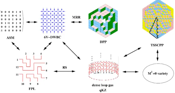
much largericeberg (see Fig.3), which

on

the

purecombinatoricssideinvolvesother objects: the$s(\succ$called

TSSCPPs

(TotallySymmetric

Self-ComplementaryPlanePartitions)which

are

yetanother kind ofplanepartitions, with

a formulation intermsofdifferent configurations ofnon-intersectinglatticepaths (seefor

instance [6] for a detailed account). There is also a statisticalphysics side, involving the

so-called Fully Packed Loop (FPL) model

on

a square grid, whose configurations

are

in

bijection with those ofthe $6V$-DWBC model. The latter plays acentral role in the

so-called Razumov-Stroganov (RS) conjecture [23] proved by Cantini-Sportiello [7], relating

its refined enumeration according to link patterns ofconnectionsof theloops around the

grid to the asymptotic probabilities of connections of the Densely Packed Loop (DPL)

MRR ASM $6V$_-DWBC $\backslash$ $\nearrow$ $12\neg$ $\underline{RS}$ $11^{-}10\rceil\overline{L}1_{-}^{-}L_{7}8$

dense loopgas

FPL _$qKZ$

Figure 3: From left to right: ASM, $6V$_{-DWBC and FPL, all in bijection; dense loop gas (DPL): its}

ground-state/limiting probability vector satisfies the$qKZ$equation, the componentsmeasureFPLcorrelations (RS

con-jecture),theirsummatchesthe$6V$-DWBC_{partitionfunctionwith inhomogeneous spectral parameters}$z.,$$w_{j}$and

$q^{3}=1$; DPPs: their refined evaluation matches that of ASMs(MRR conjecture); TSSCPPs: their refined

enu-merationmatchesa sumrulefor$qKZ$solutions atgeneric$q$and$z_{i}=1$; Variety$M^{2}=0$: its degree/multidegree

matches solutions of$qKZ$for$q=1.$

lattice modelbasedon somepictorial representationof the Temperley-Lieb algebra, whose

groundstate vector is

a

solution to thequantumKnizhnik-Zamolodchikov $(qKZ)$ _equation

[9, 10]. Finally,thereisanalgebraic geometryside of the iceberg. Forinstance, thedegree

of thevariety ofuppertriangular complex matriceswithvanishingsquare corresponds to

a refined enumeration of TSSCPPs, and the (equivariant cohomology) multidegree is

obtained via aspecialization ofthesolution to the $qKZ$equation [11].

Many of the known enumerations of the above objects involve determinants,. In a

number of cases, these

can

be obtained throughsomeapplicationof the

Lindstr\"om-Gessel-Viennot theorem. This applies to all the “free fermion”’ cases that are in bijection with

non-intersecting lattice path configurations. However, both the $6V$ model and the DPL

model

are

models ofinteracting fermions, in which even if there is

some

kind of lattice

pathformulation, the latter

are

nolonger just non-intersecting. For instance, in the

case

of the $6V$ model, one can define _{paths going from the left border ofthe grid to the top}

border, by going right and up along the oriented edges

as

much

as

possible (i.e. when there

isachoice, alwaysgo up). Suchpathsare now “osculating” in that two pathscanbounce

against each other at avertex (the first going right, then up; the second going up then

right; thiscorresponds tothevertex$a_{1}$ of the $6V$model), and thisconfigurationreceives a

differentweight, interpreted

as

theexponentialof

some

interaction

energy.

Yet, somehow,

our formula for the refined enumeration has magically disentangled this interaction, to

make it look like a free fermionmodel, via our determinant evaluation. This mechanism

6.2

Integrabilities

The$6V$model is thearchetypeof$2D$ integrablelatticemodel, related to the $1D$quantum

XXZspinchainfor $sl_{2}$. It isknowtohave

an

infinite family of transfermatrices $T(a, b, c)$

provided theBoltzmann weights $a,$$b,$$c$satisfy the followingrelation:

$\Delta(a, b, c)=\frac{a^{2}+b^{2}-c^{2}}{2ab}=$const.

This constant is the anisotropy of the associated quantum spin chain. Alternatively, in

terms ofthe $x,$$y$ variables of (3.2), thisturns into the following $(6V$

’

variety:

$\psi(x, y)=\frac{1+y-x}{\sqrt{y}}=$ const. (6.1)

as

$x,$$y>0.$

On the other hand, the infinite matrix $M_{ASM}$, whose finitely truncated determinant

gives the

DWBC

homogeneous$6V$partitionfunction

on a

grid of

same

size, alsoinvolves

a

transfer matrix$\theta$

of

a

formanalogousto thatof$1+1D$Lorentzian triangulations, generated

by:

$f_{\theta}(u, v)=\overline{1-xu-vx)uv}$

Thetransfermatrices$\theta$ commutefor different values ofthe parameters

$x,$$y$provided they

belong to thefollowing “Lorentzian” variety:

$\varphi(x, y)=\frac{1+x-y}{\sqrt{x}}=$const. (6.2)

obtainedby rephrasing (2.4) above.

Comparing (6.1) and (6.2),

we

see

that $\varphi(x, y)=\psi(y, x)$, hence the two varieties

are

distinct! However, theydo intersect. Solving for $\varphi(x, y)=q+q^{-1}$ and $\psi(x, y)=p+p^{-1}$

with say $q,p>1$, we findthat

$\sqrt{x}=\frac{p(q^{2}-1)}{p^{2}q^{2}-1} \sqrt{y}=\frac{q(p^{2}-1)}{p^{2}q^{2}-1}$

Conversely, anysuch pointfor$p,$$q>1$ liesattheintersectionoftwo “integrable varieties

of the form (6.1) and (6.2). This intriguing fact deserves a better understanding. In

particular, the $6V$variety involves commutation of

finite

size transfermatrices, whereas

the Lorentzian

one concern

matrices of infinite size.

A

Infinite

matrices

and truncated

determinants

Throughout thesenotes,

we

makeextensive

use

ofgeneratingfunctionsfor infinite

A.l Infinite matrices

We consider infinite matrices $A=(a_{i,j})_{i,j\in z_{+}}$. The very concept of an infinite matrix is

a bit delicate to work with, for instance the product oftwo such matrices might not be

well defined. This may be repaired by introducing a formal expansion parameter $\epsilon$, and

associating to$A$the matrix$A(\epsilon)=(\epsilon^{i+j}a_{i,j})_{i,j\in \mathbb{Z}+}$

.

The product ofany twosuch matrices

now

makes

sense

in the

sense

of formal power series of $\epsilon$. Moreover,

even

the notion of

eigenvector and eigenvalue make sense in this setting, provided one can show that the

latter have formal poweror Laurent series expansions in $\epsilon.$

Such aconstructionwill alwaysbeimplicit (whennot explicit) throughout these notes.

For instance, the parameter$g$in $T(g, a)$ of(2.2-2.3) playsthe roleof$\epsilon$. The

(diagonaliza-tion” of$T(g, a)$ along the integrable variety $\varphi(g, a)=q+q^{-1}$ (see Sect.2.3) is

an

example

of such extended notions ofeigenvectors and eigenvalues.

A.2 Generating functions for infinite matrices

For an infinite matrix $A=(a_{i,j})_{i,j\in z_{+}}$ and a vector $w=(w_{i})_{i\in z_{+}}$ we define the formal

generating functions

$f_{A}(u, v)= \sum_{i,j\in \mathbb{Z}+}a_{i,j}u^{i}v^{j} f_{w}(u)=\sum_{i\in z_{+}}w_{i}u^{i}$

with the following properties formatrices $A,$ $B$ and a vector $w$:

$fi(u, v) = \frac{1}{1-uv}$

$f_{A^{t}}(u, v) = f_{A}(v, u)$

$f_{Aw}(u) = \oint\frac{dt}{2i\pi t}f_{A}(u, t^{-1})f_{w}(t)$

$f_{AB}(uv) = (f_{A}*f_{B})(u, v)= \oint\frac{dt}{2i\pi t}f_{A}(u, t^{-1})f_{B}(t, v)$

where thecontour integral picks the constant term in $t.$

We consider the lower and upper triangularmatrices $L(\alpha, \beta)$ and $U(\alpha, \beta)$ with

gener-ating functions

$f_{L(\alpha,\beta)}(u, v)= \frac{1}{1-\beta u(1+\alpha v)}$ $f_{U(\alpha,\beta)}(u, v)= \frac{1}{1-\beta v(1+\alpha u)}$ (A.1)

with $U(\alpha, \beta)=L(\alpha, \beta)^{t}$

.

Let

us

also introduce the shift matrix $S=(\delta_{i,j+1})_{i,j\in \mathbb{Z}+}$ and the

transfer matrix$T(\alpha, \beta, \gamma)$ generated respectively by:

$f_{S}(u, v)= \frac{u}{1-uv}$ $f_{T(\alpha,\beta,\gamma)}(u, v)= \frac{1}{1-\alpha u-\beta v-\gamma uv}$ (A.2)

Inparticular, we have

The

case

of the infinite transfermatrix $T(g, a)$ for Lorentzian triangulations corresponds

to theidentification:

$T(g, a)=T(ga, ga,9^{2}(1-a^{2})$

We have the following properties easily derived by contour integrals for the

correspond-inggeneratingfunctions:

$L(\alpha, \beta)L(\alpha’, \beta’)$ $=$ $L( \frac{\alpha\beta’\alpha’}{1+\alpha\beta}, \beta(1+\alpha\beta’))$ (A.3)

$U(\alpha, \beta)U(\alpha’, \beta’)$ $=$ $U( \frac{\alpha\beta\alpha’}{1+\alpha\beta},\beta(1+\alpha’\beta))$ (A.4)

$L( \alpha, \beta)^{-1}=L(-\frac{1}{\beta}, -\frac{1}{\alpha})$ $U( \alpha, \beta)^{-1}=U(-\frac{1}{\beta}, -\frac{1}{\alpha})$ (A.5)

$L(\alpha, \beta)U(\alpha’, \beta’)$ $=T(\beta, \beta’, \beta\beta’(\alpha\alpha’-1))$ (A.6)

$U(\alpha’, \beta’)L(\alpha, \beta)$ $=$ $\frac{1}{1-\beta\beta’}T(\frac{\alpha’\beta\beta’}{1-\beta\beta’}, \frac{\alpha\beta\beta’}{1-\beta\beta’}, \frac{\alpha\alpha’\beta\beta’}{1-\beta\beta’})$ (A.7)

$T(\alpha, \beta, \gamma)T(\alpha’,\beta’, \gamma’)$ $=$ $\frac{1}{1-\beta\alpha}T(\frac{\alpha+\gamma\alpha’}{1-\beta\alpha’}, \frac{\beta’+\gamma’\beta}{1-\beta\alpha}, \frac{\gamma\gamma’-\alpha\beta’}{1-\beta\alpha})$ (A.8)

$T(\alpha, \beta,\gamma)^{-1}$ $=$ $\frac{\gamma}{\alpha\beta+\gamma}T(-\frac{\alpha}{\gamma}, -\frac{\beta}{\gamma}, \frac{1}{\gamma})$ (A.9)

These hold whenever the denominators

are

non-vanishing.

A.3 Commuting families and addition formulas

Using the

formulas

above, it is easy to derive the following:

Theorem A.l. The following family $\{T_{s,t}(\alpha)\}_{a\in C}$

of infinite

matrices commute among

themselves

_for

any

_fixed

values

_of

$s$ and$t$:

$T_{s,t}(\alpha)=T(\alpha, s\alpha, 1-t\alpha)$

Wealso have the following “addition formula:

$T_{s,t}( \alpha)T_{s,t}(\alpha’)=\frac{1}{1-s\alpha\alpha’}T_{s,t}(\frac{\alpha+\alpha’-t\alpha\alpha’}{1-s\alpha\alpha’})$

For$s=0$, we obtainafamilyofcommuting lower triangular matrices

$L_{t}( \alpha)=T_{0,t}(\alpha)=L(\frac{1}{\alpha}-t, \alpha)$

with the (addition” _formula:

$L_{t}(\alpha)L_{t}(\alpha’)=L_{t}(\alpha+\alpha’-t\alpha\alpha’)$

Changing variables from $\alpha$to $a$, with$\alpha=\frac{1-e^{-ta}}{t}$, and writing$\ell_{t}(a)=L_{t}(\alpha)$ wefinally get

the addition formula:

from which

we

deduce that $\ell_{t}(a)$ is

an

infinitematrix exponential. Moreprecisely, let $M_{t}$

be the infinite matrix generated by

$f_{M_{t}}= \frac{(tv-1)u}{(1-uv)^{2}} M_{t}=(^{\frac{0}{00}1} \frac{0t}{0}2 -32t00 ..3t\cdots)$

then we have $\ell_{t}(a)=\exp(-aM_{t})$, which by triangularity holds for any finite truncation

as well. A similar analysis holds for $T_{s,t}(\alpha)$, but only for the infinite matrix. Assuming

that $t^{2}-4s>0$_{, and introducing another parameter} $r=\sqrt{1-4s}/t^{2}$, the relevant change

ofvariables is:

$\alpha=\frac{2(e^{rta}-1)}{t(te^{rta}(r+1)+r-1)} \tau_{r,t}(a)=T_{s,t}(\alpha)$

in termsofwhich

$\tau_{r,t}(a)\tau_{r,t}(a’)=\frac{1}{1-\frac{(1-r^{2})(e^{rta}-1)(e^{rta’}-1)}{(te^{rta}(r+1)+r-1)(te^{rta’}(r+1)+r-1)}}\tau_{r,t}(a+a’)$

This reduces to (A.10) when$r=1$ (corresponding to $s=0$).

A.4 Truncated determinants

For anyinfinite matrix$A=(a_{i,j})_{i,j\in z_{+}}$,we denote by $A^{[0,n-1]}$ the finite$n\cross n$ truncation of

$A$to its$n$firstrowsand columns, namely the matrix with entries: $A^{[0,n-1]}=(a_{i,j})_{i,j\in[0,n-1]}.$

In general, the matrixproduct does not respect truncation. However, if$L,$ $U$ are

re-spectively lowerandupper triangularinfinitematrices, then $(LU)^{[0,n-1]}=L^{[0,n-1]}U^{[0,n-1]}.$

Note that this does not hold for $(UL)$ (see theexample below).

Let us

now

examinetruncated determinants, namelythe determinant of such finitely

truncated matrices. By triangularity it is immediate tocompute:

$\det(L(\alpha, \beta)^{[0,k]})=(\alpha\beta)^{k(k+1)/2}=\det(U(\alpha, \beta)^{[0,k]})$ (A. 11)

and bythe above propertywe deduce from (A.6) and (A.11) that:

$\det(T^{[0,k]}(\beta, \beta’, \beta\beta’(\alpha\alpha’-1 =\det(L(\alpha, \beta)^{[0,k]}U(\alpha’, \beta’)^{[0,k]})=(\alpha\beta\alpha’\beta’)^{k(k+1)/2}$

and more generally

$\det(T^{[0,k]}(\alpha, \beta, \gamma))=(\alpha\beta+\gamma)^{k(k+1)/2}$

whereas

$\det((U(\alpha’, \beta’)L(\alpha, \beta))^{[0,k]}) = \frac{\det(T^{[0,k]}(\frac{\alpha’\beta\beta’}{1-\beta\beta’},\frac{\alpha\beta\beta’}{1-\beta\beta},\frac{\alpha\alpha’\beta\beta’}{1-\beta\beta}))}{(1-\beta\beta’)^{k+1}}$

by

use

of (A.7). The discrepancy with the$LU$

result

is because the matrix product

now

involves all theelementsof the $(k+1)\cross$ infiniteand infinite $\cross(k+1)$ rectangularmatrices

of the truncated product.

Themainproperty allowingforprovingtruncateddeterminant identities from relations

between generatingfunctions is thefollowing:

Lemma A.2. Let$L,$ $U,$ $A$ be respectively lower triangular, upper triangular and arbitrary

infinite

matrices, and let $M=LAU$. Then:

$M^{[0,k]}=L^{[0,k]}A^{[0,k]}U^{[0,k]}$

Assuming further that both$L$and$U$areunitriangular,wethendeducethat$\det(M^{[0,k]})=$

$\det(A^{[0,k]})$ for all $k\geq 0$

.

So

we

will have identity between all truncated determinants of

two infinite matrices $M$ and $A$if there is a relation $M=LAU$ for $L,$ $U$ lower and upper

unitriangular infinite matrices. References

[1] G. Andrews, Plane partitions. III. The weak Macdonald conjecture, Invent. Math.

53 (1979), No. 3, 193-225 and Macdonalds conjecture and descending plane

parti-tions, Combinatorics, representation theory and statistical methods in groups,

Lec-tureNotesin Pure and Appl. Math., vol. 57, Dekker, New York, (1980), pp. 91-106.

[2] J. Ambjorn andR. Loll, Non-perturbativeLorentzian quantum gravity, causality and

topology change Nucl. Phys. B536 (1998) 407-434.

[3] M.T. Batchelor, J. de Gier and B. Nienhuis, The quantum symmetric XXZ chain

at $\Delta=-1/2$, alternating sign matrices and plane partitions, J. Phys. A34 (2001)

L265-L270. $cond-mat/0101385.$

[4] R. Behrend, P. Di Francesco and P. Zinn-Justin,

On

the weighted enumeration

_of

AlternatingSign Matrices andDescendingPlane Partitions. J. Combin. TheorySer.

A119 (2) (2012), 331-363. arXiv:1103.1176.

[5] R. Behrend , P. Di Francesco and P. Zinn-Justin , The doubly

_refined

enu-meration

_of

Alternating Sign Matrices and Descending Plane Partitions. (2012),

arXiv:1202. 1520.

[6] D. Bressoud,

_Proofs

and

_{confirmations:}

The story

_of

the alternating sign matrix

conjecture, MAA Spectrum, MathematicalAssociation ofAmerica, Washington,DC

(1999), 274 pages.

[7] L. Cantiniand A. Sportiello,

_{Proof of}

the Razumov-Stroganovconjecture, Journal: J.

Comb. Theory A118 (2011)

1549-1574.

arXiv:1003.3376.

[8] P. Di Francesco, E. Guitter, andC. Kristjansen, Integrable2D Lorentziangravity and

[9] P. DiFkancesco andP. Zinn-Justin, Around the Razumov-Stroganovconjecture: proof

of

a

multi-parameter

sum

rule. Electron. J.

Combin.

12 (2005), Research Paper 6,

27

pp. arXiv:$math-ph/0410061.$

[10] P. Di Francesco and P. Zinn-Justin, Quantum Knizhnik-Zamolodchikov Equation,

Totally Symmetric Self-Complementary Plane Partitions and Alternating Sign

Ma-trices. Theor. Math. Phys. 154 (3) (2008), 331-348. arXiv:$math-ph/0703015.$

[11] P. Di Francesco and P. Zinn-Justin, Quantum Knizhnik-Zamolodchikov equation,

generalizedRazumov-Stroganovsumrules and extendedJoseph polynomials, J. Phys.

A: Math. Gen. 38 (2005) L815-L822. arXiv:$math-ph/0508059$

[12] C. Dodgson, Condensation

_of

determinants, Proceedingsof the RoyalSoc. of London

15 (1866) 150-155.

[13] S. Fominand A. Zelevinsky Cluster Algebras I. J. Amer. Math. Soc. 15 (2002), no.

2,

497-529

arXiv:$math/0104151$ [math. RT].

[14] I. M. Gessel and X. Viennot, Binomialdeterminants, paths and hook formulae, Adv.

Math. 58 (1985)

300-321.

[15] A. Izergin, Partition

_{function of}

the six-veriex model in a

_finite

volume, Sov. Phys.

Dokl. 32 (1987) 878-879.

[16] A. Knutson, T. Tao, and C. Woodward, A positive proof

_of

the

Littlewood-Richardson rule using the octahedron recurrence, Electr. J. Combin. 11 (2004) RP

61. arXiv:$math/0306274$ [math.

_C01

[17] V. Korepin, Calculation

_of

norms

_of

Bethe wavefunctions, Comm. Math. Phys. 86

(1982) 391-418.

[18] G. Kuperberg, Another proof

_of

the alternating-sign matrix conjecture, Int. Math.

Res. Notices No 3 (1996)

139-150.

arXiv:$math/9712207.$

[19] P. Lalonde, Lattice paths and the antiautomorphism

_of

the poset

_of

descending plane

partitions, Discrete Math. 271 (13) (2003) 311-319.

[20] C. Krattenthaler, Descending plane partitions and rhombus tilings

_of

a hexagon

with a triangular hole, European J. Combin. 27 (7) (2006) 1138-1146.

arXiv:$math/0310188.$

[21] B.Lindstr\"om, On the vectorrepresentations

_of

inducedmatroids, Bull.London Math.

Soc. 5 (1973) 85-90.

[22] W. H. Mills,D. P.Robbins, and H. Rumsey, Alternatingsignmatrices and descending

plane partitions, J. Combin. Theory Ser. A 34 (1983), 340-359.

[23] A.V. Razumov and Yu.G. Stroganov, Combinatorial nature

_of

ground state vector

_of

0(1) loopmodel, Theor. Math. Phys. 138 (2004) 333-337; Teor. Mat. Fiz. 138(2004)

[24] W. Mills, D. Robbins, H. Rumsey Jr.,

_Proof

of

the Macdonald conjecture, Invent.

Math.66(1) (1982) 73-87; D. RobbinsandH. Rumsey, Determinants andalternating

sign matrices, Adv. Math. 62 (1986),

169-184.

[25] D. Zeilberger,

_{Proof of}

the alternating sign matri

x

conjecture, Elec. J. Comb. 3 (2)

(1996), R13.

Institut de Physique Th\’eorique duCommissariat \‘a l’Energie Atomique,

Unit\’e deRecherche associ\’eedu CNRS,

CEA Saclay/IPhT/Bat 774,F-91191 Gif

sur

Yvette Cedex,

FRANCE.