Geometric Characterizations of Standard Normal Distribution : Two Types of Differential Equations, Relationships with Square and Circle, and Their Similar Characterizations (Decision making theories under uncertainty and its applications : the extensions

全文

(1)58. 数理解析研究所講究録第2078巻 2018年 58-64. Geometric Characterizations of Standard Normal Distribution ‐ Two Types of Differential Equations, Relationships with Square and Circle, and Their Similar Characterizations‐ and. Shingo NAKANISHI. Masamitsu OHNISHI Graduate School of Economics and. Center for Mathematical Modeling and Data Science, Osaka University. Computing Center, Osaka Institute of Technology 1. Introduction. We confirm various kinds of geometric characterizations of a standard normal distribution with Pearson’s finding probabilistic point 0.612003 and its cumulative probability 0.2702678 on a standard normal distribution [1]. After Pearson proposed that, their numbers were studied by Kelley [2, 3], Mosteller [4], Cox [5] and many researchers [6‐12]. Our studies [13‐17] are also some ofthem. Sclove [6, 7] explained Cox’s proposal to us as the clustering ofnormal distribution. Nakamori et al [8] also mentioned that Cox’s proposal was one of the original papers of \mathrm{K} ‐means Algorisms. Kelley’s formulation, $\phi$( $\lambda$)=2 $\lambda \Phi$(- $\lambda$) , is also known as the 27 percent rule [9‐12]. We found the other characterizations about 0.612003 from the parabolic curves ofthe cost ofthe repetitions game ofcoin tossing [13] and the square on a standard normal distribution with the probabilistic point 0.612003 [14‐17]. In this paper, we confirm several characterizations based on this paper title. First, we show the geometric characterizations both Bemoulli differential equations [18] of inverse Mills ratios [19, 20] as the hazard functions and survival functions on standard normal distributions. At the same time, we find that Pearson’s 0.612003 should be also an important role in their relations. Second, we clarify that variable coefficient second‐order linear homogeneous differential equations [21] are related to a standard normal distribution. Especially, Sturm‐Liouville form [22] with a probability density function ofa standard normal distribution is shown concisely. Moreover, we illustrate that the value 0.612003 shows the curve which is the integral form of the cumulative distribution has the tangent lines on essential key points. Furthermore, we also find the similar tendencies from European and Oriental historical cultures about the relations close to theology between circles and squares. Coincidentally, we get a practical approximated value 0.612004 from an equilateral triangle on the geometric characterization between circles, squares and a standard normal distribution instead of Pearson’s finding true value 0.612003.. 0.0. 00. (a) Typc of a triangular distribution \prime. (b) Typc of a unifonn distribution. 00. (c) Typc ofan cxponcntial distribution. /. Our concepts are shown as mtegral forms of cumulative distnbution imctions. CJreen dashed lines are probability density functions (\mathrm{P}\mathrm{D}\mathrm{F}):J(x) , Red dashed lines are cumulative distribution functions (CDF): F(x) , Purple 1‐dot chain lines are Integrals of each cumulative distribution fimctlon, Red dotted lmes are 1 0, Purple dotted lines are asymptotuc lmes whose slopes are 10.. Aspect ratio =10. Figure 1 Concepts of integral forms of various kinds of cumulative distribution functions and their probability density functions. (a) Triangular distribution, (b) Uniform distribution, (c) Exponential distribution and (d) Standard normal distribution. 2. Our Concepts of This Study Prof. Sandoh who was one oftwo referees ofthe first author’s doctoral thesis [14] advised us to reconfirm the calculations. practically about our previous research [13, 14] such as a general integral form [23]. We reconsider that as the following equation. E(U| <-$\lambda$)=\displayst le\frac{\int_{-\infty}^{-$\lambda$}u$\phi$(u)du}{\int_{-\infty}^{-$\lambda$} \phi$(u)du}=-\frac{$\phi$( \lambda$)}{$\Phi$(-$\lambda$)}=-2$\lambda$. (1). as well as using the regression analysis [13, 14]. $\phi$(u) is a probability density function of a standard normal distribution on.

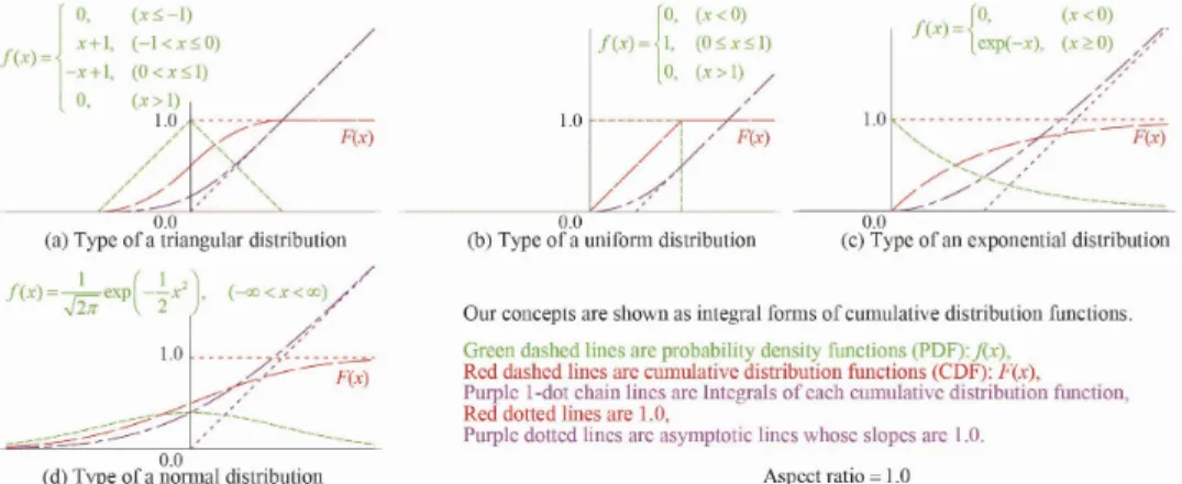
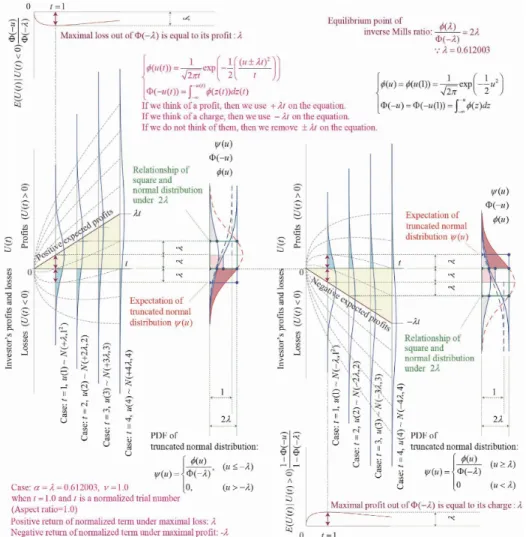
(2) 59. its probabilistic point \mathrm{u}. $\Phi$(- $\lambda$) is a calculated value of a cumulative distribution function from -\infty to - $\lambda$ on u. $\lambda$ that is about 0.612003 should be an important role ofthis study on u. $\phi$(u)/ $\Phi$(-u) is an inverse Mills ratio [19, 20]. Prof. Oya who was the other referee recommended us to investigate the tendencies between squares and normal distributions about our previous research [14]. We think oftwo precious advices as the concepts such as the integral forms of cumulative distribution functions like an idea by Nagasaka, Tsukamasa and Hashimoto [24] in Figure 1. That is, several putple 1‐dot lines are shown. in Figure 1. In this study, we clarify that the curve of an integral form ofa cumulative distribution function of standard normal distribution has a principal role such as two types of differential equations and passes through several crucial points on their equations in this paper. By the way, Kelley also proposed the 27 percent rule formulation about $\lambda$=0.612003 as follows. \displayst le\frac{$\phi$( \lambda$)}{$\Phi$(- \lambda$)}=2$\lambda$. from. \displaystyle \frac{d $\phi$(u)}{d\mathrm{u} =-u $\phi$(u) and \displaystyle \frac{d $\Phi$(-u)}{du}=- $\phi$(u) .. (2). At this time, we show that the fact, $\phi$( $\lambda$) is equal to 2 $\lambda \Phi$(- $\lambda$) from Equations (1) and (2), brings us the equilibrium points in Figure 2. That is to say, a positive retum is equal to its standard deviation as maximal loss [16, 17] and a negative return is equal to that as maximal profit [13‐15, 17] under the condition that has the expected value as $\lambda$ and its standard deviation 1.0 in Figure 2. From Figure 2, we confirm that the square whose length is 2 $\lambda$ is an expected value of a truncated normal distribution [25].. \chek{mathr{e}\wdgaprox|. \hat{\mathrm{o} \vee. -\underli{\mathrb}\prox. \chek{\mathrm{b}\sim \tilde{\mathrm{k}). \dot{mathrm{b}\wedg\sim. \underli{matho}\infy{$ t} \triangleft\mahr{c}\triangleft. \displaytefrc{.\undlieB}mathr{o,\d ma}. \displaytefrc{.omh}undi\tsberaglfy>}. Ca. \mathrm{w}\}. (\mathrm{A} \mathrm{p}_{0}. Negative retum ofnormalized term under maxumal profit:. Figure 2. - $\lambda$. \mathrm{r}\triangle ft. 0. t=1. Equilibriun points both positive or negative returns and their risks under the condition on a standard nonnal distribution ( $\lambda$=0.612003, \mathrm{t}=1.0 , Original reference [17.

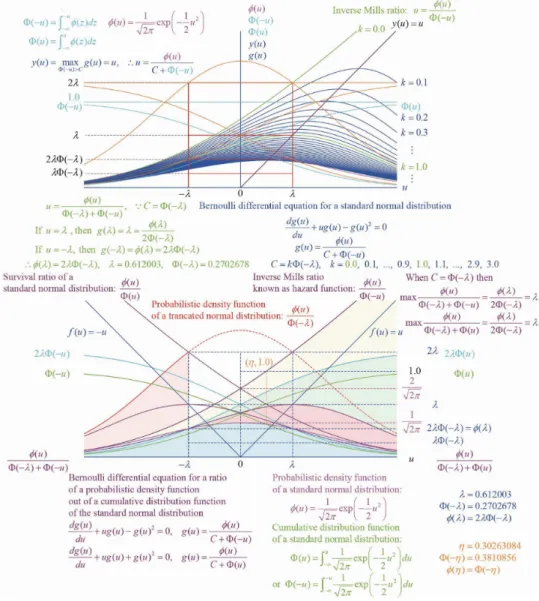
(3) 60. Especially, our concept about a negative return is similar to the meaningful insists of both Prof. Watanabe’s website [26] and Prof Tanioka’s textbook [27] as the fee of gambling. On the other hand, the other about a positive return is similar to the general thinking about that a capital return is greater than its growth return historically such as Piketty’s proposal [28]. 3. Bernoulli Differential Equations for Inverse Mills Ratio In section 2, we confirm that the equilibrium points on a standard nornal distribution are shown based on $\lambda$=0.612003.. According to Isa’s research [20], we rethink of the following formulations as Bemoulli differential equation with a standard normal distribution when we consider the tendencies of an inverse Mills ratio and a hazard function as the special cases on $\lambda$. The equation such as Bernoulli differential equation with a standard normal distribution is also mentioned in Prof. Kijima’s special lecture [18]. However, since we are interested in the geometric characterizations of that, we propose two types of homogeneous Bemoulli differential equations. That is. $\Phi$(-l )=\displaystyle \int $\Phi$ =\rfloor y(u)=. ... .,. \backslash. 1. (. 1. ). \wedge\prime\ mptyset(u)_{-} .、. \mathrm{q}. (1 2 3. 2 $\lambda \Phi$. 0. $\lambda \Phi$. u=. If. u=. If. u=. 0,. .. $\phi$( $\lambda$)= Survival ratio. 1.1,. 29, 30. |\mathrm{n}C= $\Phi$(- $\lambda$) then. \mathrm{c}. standard normé. \displaystyle\frac{$\phi$(u)}{\mathrm{D}(-$\lambda$)+$\Phi$(-u)}=\frac{$\phi$($\lambda$)}{2$\Phi$(-$\lambda$)}=$\lambda$ \displaystyle\frac{$\mu$_{u)}{$\Phi$(-$\lambda$)+$\Phi$(u)}=\frac{$\phi$($\lambda$)}{2$\Phi$(-$\lambda$)}=$\lambda$ 2 $\lambda$. 2 $\lambda \Phi$($\Phi$(-. 2 $\lambda \Phi$( $\iota$/). $\Phi$(u), $\lambda$. $\phi$(\mathrm{u}) $\Phi$(- $\lambda$)+ $\Phi$(-u). - $\lambda$ 0. $\lambda$. Bernoulh dhfferential equation for a ratio. )1. of a probabilistic dcnsity function. |1\mathrm{f} a standard normal distribution:. robabilistic density function. out of a cumulabve dtstnbution function of the standard normal distribution. \displaystyle \frac{dg(u)}{du}+ug(u)-g(u)^{2}=0, g(u)=\frac{ $\phi$(u)}{C+ $\Phi$(-u)} \displaystyle \frac{dg(u)}{du}+\mathrm{u}g(u)+g(u)^{2}=0, g(\mathrm{u})=\frac{ $\phi$(u)}{C+ $\Phi$(u)}. \neg. $\phi$(u)=\displaystyle \frac{1}{\sqrt{2 $\pi$} \exp(-\frac{1}{2}u^{2}). , umulative distribution function 1. \mathrm{f} a standard normal distribution:. \rangle \mathrm{r}. $\Phi$(u)=\displaystyle\int_{\rightar ow\urcorner}^{u}\frac{1}{\backslash^{\prime'}2$\pi$}\exp(-\frac{1}{2}u^{2})du $\Phi$(-u)=\displayst le\int_{-\infty}^{-u}\frac{1}\sqrt{2$\pi$}\exp\left(\begin{aray}{l -u^{2}\underline{\mathrm{l}\ 2 \end{aray}\right)du. 2 $\lambda \Phi$(- $\lambda$)= $\phi$( $\lambda$) $\lambda \Phi$(- $\lambda$) $\phi$(u) $\Phi$(- $\lambda$)+(\mathrm{D}(u) $\lambda$=0.612003. $\Phi$(- $\lambda$)=0.2702678 $\phi$( $\lambda$)=2 $\lambda$. $\eta$=0.30263084 $\Phi$(- $\eta$)=0.3810856 $\phi$( $\eta$)= $\Phi$(- $\eta$). Figure 3 Bemoulli differential equation ofthe ratios ofprobability density function of standard normal distribution out ofits cumulative distribution function with thinking of its truncated normal distribution on the probabilistic point $\lambda$=0.612003..

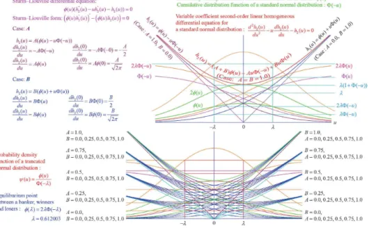
(4) 61. \displaystyle \frac{dg(u)}{du}+\mathrm{u}g(u)-g(u)^{2}. =0 ,. g(u)=\displaystyle \frac{ $\phi$(u)}{C+ $\Phi$(-u)}. \displaystyle \frac{dg(u)}{du}+ug(u)+g(\mathrm{u})^{2}=0, g(u)=\frac{ $\phi$(u)}{C+ $\Phi$(u)}. (3). .. .. (4). Based on the ideas ofasymptotic lines by Gordon [19] and Isa [20], we illustrate the Bernoulli differential equations as the geometric curves in the upper chart \mathrm{o}\mathrm{f}$\Gamma$ igure 3 with $\lambda$=0.612003 . At this time, a constant C is changed by k from 0.0 to 3.0 by 0.1 to illustrate those curves clearly. Especially, we confirn that their tendencies are shown as the special types with $\lambda$=0.612003 when k=0.0 or 1.0. Moreover, 0.30263084 that is also a probabilistic point with the same values ofboth its cumulative distribution function and probability density function is another important point because the inverse Mills ratio is equal to 1.0. Under the condition of u=0 , we fmd the inverse Mills ratio is 2 $\phi$(0)(=2/\sqrt{2 $\pi$}) as 2 times of $\phi$(0) . The lower chart also ilIustrates the geometric tendencies about Equations (3) and (4) divided by u=0 symmetrically. 4. Sturm‐Liouville Differential Equations for a Standard Normal Distribution In section 2, we mentioned our research concepts as the integral forms of a cumulative distribution of a standard normal distribution. We searched for their several characterizations [29, 30] and their differential equations about nonnal distribution [30, 31]. From our investigations, we propose the variable coefficient second‐order linear homogeneous differential equation in Figure 4. Sturn\vdashLiouville differential equation: StuimLiouville form:. Tangential equation:. $\phi$(u)(h_{l}(u)-uh_{2}'(\mathrm{u})-h_{2}(u))=0. ( $\phi$(u)h_{l}(u) '-( $\phi$(\mathrm{u})h_{2}(\mathrm{u}) =0. f(u)=\left\{ begin{ar ay}{l -(1 $\Phi$(-$\lambda$)u+2$\lambda\Phi$(-$\lambda$)&(-2\lequ\leq0)\ -$\Phi$(-$\lambda$)u+2I_{\ve }$\Phi$(-$\lambda$)&(0\lequ\leq2 \end{ar ay}\right.. Probability density function of a standard normal distnibution: $\phi$(u) Cumulative distribution function of a standard nornal distribution:. Intercept form of a linear equation for winmers :. $\Phi$(-u). -\displaystyle\frac{1}{$\lambda$}\mathrm{u}+\frac{1}{x\mathrm{D}(-$\lambda$)}$\phi$_{?}=1. Equiliburium point of an inverse Mills ratio :. Intercept form of a linear equation for losers :. \underline{1}\mathrm{u}+$\phi$_{?}\underline{1}=1. Intercept form of a lmear equation far a banker --. -\displaystyle\frac{1}{$\lambda$}\mathrm{u}+\frac{1}{$\lambda$}h=1. \displayst le\frac{$\phi$( \lambda$)}{$\Phi$(- \lambda$)}=2$\lambda$. $\lambda$(\displaystyle\frac{1+$\Phi$(-$\lambda$)}{1-$\Phi$(-$\lambda$)} $\lambda$(1+$\Phi$(-$\lambda$). Utility fUmction for winners:. U_{W}(t)=( $\phi$( $\lambda$)- $\lambda \Phi$(- $\lambda$))\sqrt{t}= $\lambda \Phi$(- $\lambda$)\sqrt{t}. Figure 4 Geometric relationships between Sturm‐Liouville differential equation and standard normal disUibution with a circle, squares, meaningful rectangles, their diagonals, and special tangent lines under $\lambda$=0.612003..

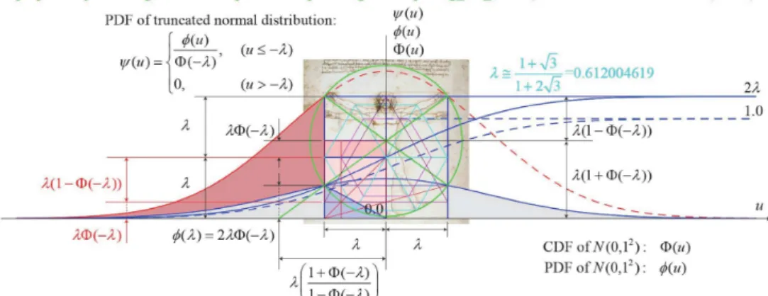
(5) 62. That is. \displaystyle \frac{d^{2}h_{2}(u)}{d\mathrm{u}^{2} -u\frac{dh_{2}(u)}{du}-h_{2}(u)=0. .. (5). The way of an expression of h_{2}(\mathrm{u}) in Equation (5) is based on the descriptions of our previous research [14]. The formulations of h_{2}(u) are shown as the following equation. h_{2}(u)=A( $\phi$(u)-u $\Phi$(-u))+B( $\phi$(u)+u $\Phi$(\mathrm{u})) .. (6). If we consider the conditions dh_{2}(u)/du=1/\sqrt{2 $\pi$} and h_{2}(u)=1/2 in Equation (5), we get the answer with A= 1.0 and B=0.0 in Equation (6). Therefore, we also confirm that the special curve in Figure 4 passes through several fundamental points with $\lambda \Phi$(- $\lambda$) and $\lambda$(1+ $\Phi$(- $\lambda$)) [17] . At the same time, we fmd their points also have the crucial tangent lines shown in Figure 4. Moreover, we illustrate a true circle with a square and a standard normal \mathrm{d}\mathrm{i}\mathrm{s}$\vartheta$ibution in Figure 4 [17]. The center ofthis circle is an intersection of meaningful rectangle diagonals. Without passing through the intersection, we fmd the other important line to distinguish into the separated squares by the proportion $\Phi$(- $\lambda$):1- $\Phi$(- $\lambda$) . We reconfirm the geometric characterizations about $\lambda$=0.612003 with considering a square, a circle and a normal distribution. And their tendencies have a special differential equation as the following Sturm‐Liouville form [22]. ( $\phi$(u)h_{2}'(u))'+( $\phi$(u)h_{2}(u))=0 . At this time, to investigate the tendencies ofthe combinations between by the values from 0.0 to 1.0 by 0.25 respectively in Figure 5.. h_{?}(u)=\mathrm{A}(\emptyset(u)-u $\Phi$(-1l)). \ve dh_{2}(u\underline{)}du.=-A $\Phi$(-u) \displaystyle \frac{dh_{2}(u)}{du}=A $\phi$(u). B. \mathrm{o}\mathrm{t}\cdot \mathrm{a}. in Equation (6),. A. and. \prime$\varsigma$:_{\mathrm{o} $\xi$_{r_{*}. Vanablcicoetficienl ’;ec.ond‐or \mathr {k}1\mathr {i}\mathfrk{n}\mathr {e}\mathr {}\mathr {}\mathr {}_\mathr {o}\mathr {m}()\ athrm{g}\ athrm{c}\ athrm{n}\ athrm{C}\ athrm{O}\ athrm{}\ athrm{L}\ athrm{s}d^2h(u\`{i}dh_-l$\iota el1 diffcrcntial $\eta$ uation for. B. are changed. standard normal dhstnbution. $\phi$(u). Cumulative distribution function of a standard normal distnbution:. $\phi$(u)\langle l_{l_{2}}(u)-uh_{2}(u)-h_{2}(u))=0. ( $\phi$(u)h_{\dot{r}_{\sim} (\mathrm{u}) -( $\phi$(u)h_{r}.(u) =0. (7). and. Probability density inction. Sturni‐Liouville differential equation:. \mathr{C}\mathr{}\mathr{s}\mathr{c}:A\mathr{S}\mathr{}$\iota-\suc mathr{L}\mathr{i}_\mathr{o}\mathr{u}\mathr{V}\mathr{i}1\mathr{e} form:. A. $\Phi$(-u). $\varthe$^{\Phi$^{\backsl h$\varthe$_{\sim}^{\backsl h} /\backslah^{\mathrm{s}\backslah}. \displaystyle \frac{dh_{\angle}(0)}{du}=-A $\Phi$(-0)=-. \displaystyle\frac{dh_{2}(0)}{d\mathrm{u}=r1$\phi$\langle0)=\frac{A}{\sqrt{2$\pi$}. \mathrm{t})(u) $\Phi$(u). Case: B. (|- $\Phi$(-u)) h_{2}(u)=B( $\mu$ u)+u $\Phi$(u)). \displaystyle \frac{dh_{2}(u)}{du}=B $\Phi$(\mathrm{u}) \displaystyle\frac{dh\underline{},($\iota$r)}{du}=B$\phi$(\mathrm{u}). \displaystyle \frac{dh_{2}(0)}{du}=B $\Phi$(0)=\frac{B}{2}. $\Phi$(-u). \displaystyle \frac{dh_{2}(0)}{du}=B $\phi$(0)=\frac{B}{\sqrt{2 $\pi$}. $\Phi$(-u). A=1.0, B=0.0 ,. Probabihty density funcbon of a trancated normal distnbution :. $\psi$(|p)=\displayst le\frac{$\phi$(\mathrm{u}){\fcir le(-$\lambda$)} Equffiburium pomt betwecn a bankcr, wmncrs. arid losers : Of $\lambda$ ) =2 $\lambda \Phi$(- $\lambda$) $\lambda$=0.612003. Figure 5. 0.25, 0.5, 0.75, 1.. |0.75 , 1.0. A=0.75, B=0.0 , 0.25, 0.5. 0.75, 1.. , 0.75, 1.0. A=0.5, B=0.0 , 0.25.0.5. 0.75, 1.. .0.75, 1.0. A=025, B=0.0 , 0.25, 0.5, 0.75, 1.. , 0.75, 1.0. A=0.0, B=0.0 , 0.25, 05, 0.75, 1.. , 0.75, 1.0. Various geometric characterizations of Strum‐Liouville differential equations with standard normal distribution.. 5. Square and Circle on Standard Normal Distribution and Approximated Vałue about Polygons Although we confirm that there is a relationship between a circle, a square and a normal distribution, we cannot get a correct value $\lambda$ as well as drawing an equilateral triangle and a regular hexagon from their characterizations which are similar to the problem of squaring the circle [32, 33]. Instead ofthat, we can get the practical approximated Pearson’s findin\mathrm{g} value. That is. $\lambda$\displaystyle \cong\frac{1+\sqrt{3} {1+2\sqrt{3} =0.6120 4. .. (8). This approximated value is estimated by drawing equilateral triangles and regular hexagons shown in Figure 6. By the way, there are a lot ofthinking about circles and squares for a long time all over the world religiously and historically [32‐39]. We also show one oftheir tendencies with a standard normal distribution based on $\lambda$=0.612003 . Coincidentally,.

(6) 63. since its value is close to an inverse of golden ratio, we illustrate an imitated figure like one of da Vinci’s works “Vitruvian Man” [34.35] and based on “Mandalas” [36, 37]. According to Prof. Ida’s opinion, it is said that the proportion ofthat by da Vinci should be less than the inverse ofgolden ratio (\cong 0.618) slightly. From oriental areas to western areas, there are many theological cultures about circles and squares. And from Egyptian civilization to Greek era and Roman era, the normal distribution had not been known before De Moivre (1733), Laplace (1812), Legendre (1805), and Gauss (1809) studied it [38,39]. At that time of Renaissance era, it is said that da Vinci was interested in the golden ratio, the Fibonacci number, and theology about squares and circles. Originally, mathematics and statistics have been developed in search of scientific evidences for the development ofbusiness, politics, sociology, life science, technology and any other fields for happiness of human beings. In order to pursue that, we propose their geometric characterizations ofthe standard normal distribution in this paper. We estimate the practical approximated value such as “Squaring the circle” which is simmilar to a problem proposed by ancient geometers. https: / \mathrm{e}\mathrm{n} .wikipedia.org wiki /\mathrm{S}\mathrm{q}\mathrm{u}\mathrm{a}\mathrm{n}\mathrm{n}\mathrm{g}_{-}\mathrm{t}\mathrm{h}\mathrm{e}_{-} circle (Access date: November 18th, 2017). Our concept ofthe integration of standard normal disribution with a square and a circle is similar to “Mandala” and \mathrm{c}. ‘Vitruvian Man” which is one of da Vinci’s works coincidentally. The oniginal reference websites are. \mathrm{h}0\mathrm{p}\mathrm{s}:/ \mathrm{e}\mathrm{n} .wihpedia.org /\mathrm{w}\mathrm{i}\mathrm{h}/Mandala, \mathrm{h}\mathfrak{n}\mathrm{P}\mathrm{s}:/ \mathrm{i}\mathrm{a} .wihpedia.org/\dot{\mathrm{w} \mathrm{k}\mathrm{i}/ 曼茶羅,. https:ljen.wihpedia.orywikifViffuvian-\mathrm{M}\mathrm{a}\mathrm{n} (Access date: July, 3\mathrm{t}\mathrm{h} , 2017).. Moreover, we are able to refer the idea and figure of Prof. Ida’s website which is discribed that the ratio should be less than the inverse number of the golden ratio. Reference: Ida, \prime1^{\backslash}. , “Vitmvian Man by Leonardo da Vinci and the Golden Ratio. http: / \mathrm{w}\mathrm{v}\cap \mathrm{v} . crl.nitech. ac.\mathrm{j}_{\mathrm{P}^{f'}}\prime. .html (Access date: July,. 3\mathrm{t}\mathrm{h} ,. 2017).. Figure 6 Approximated value of $\lambda$=0.612003 on the standard normal distribution which associates with the equilateral triangles and hexagons based on the squaring the circle with da Vinci’s work. 6. Conclusions. In this paper, we deal with the geometric characterizations about a standard normal distribution. First, we clarify that the inverse Mills ratio shown by Pearson’s finding value 0.612003 is formulated as Bernoulli differential equations. Second, we confirm that the integral form of a cumulative distribution function of standard normal distribution is expressed as Sturm‐Liouville differential equation. Third, although we admit we cannot draw a equilateral triangle correctly, we estimate the approximated value 0.612004 and illustrate the similar chart which is our mathematical concept about da Vinci’s art “Vitruvian Man”’ and “Mandalas.” Finally, we realize that the true height of densities of a standard normal distribution is much smaller than we thought of that shown in many textbooks under the aspect ratio is 1.0 throughout this study. Acknowledgments. 本研究の発表に至るまでに,[13] の覆面論文査読者2名の先生,三道弘明先生,大屋幸輔先生,渡辺隆裕先生,田畑吉雄先生,寺岡義伸先生,仲川勇二先生,木島正明先生,穴太克則先生,黒沢健先生,長塚豪己先生,堀口正之先生,西原理先生,蓮池隆先生をはじめ,OR 学会の先生方から多くの助言や知見を頂きました.ここに謝意を表します.また,第一著者の中西真悟は若い頃の恩師中易秀敏先生,栗山仙之助先生と,リスクと確率論について手解きしてくれた若い頃の上司亀島紘. 二先生,志垣一郎先生に感謝します.加えて特に,第一著者が[13] に取組んだ時から本論文作成までに,何度も繰り返しじゃんけんの勝敗の行方を楽しみ,一緒に寺社を巡り,傍で社会科に興味を持ちながら,自力で算数の問題を解くために一生懸命に補助線を描いていた第一著者の愛娘に感謝します.最後に,本研究には大阪工業大学研究奨励金による経済的支援を受けたこと.

(7) 64. を記します. References. [1] [2] [3] [4] [5] [6] [7] [8]. Pearson, K., “On the probable errors of frequency constants”, Biometrika, 13, 113‐32, (1920). Kelley, T. L., ”Footnote 1] to Jensen, MB, Objective differentiation between three grouPs in education (teachers, research workers, and administrators Genetic psychology monographs, 3(5), 361, (1928). Kelley, T. L., “The selection of upper and lower groups for the validation oftest items Journal ofEducational Psychology, 30(1), 17‐24 (1939). Mosteller, F., “On Some Useful lnefficient Statistics The Annals ofMathematical Statistics, 17, 377‐408, (1946). Cox, D. R., “Note on grouping Journal ofthe American StatisticalAssociation, 52(280), 543‐547, (1957). Sclove, S. L., A Course on Statistics for Finance Chapman and Hall /\mathrm{C}\mathrm{R}\mathrm{C} , (2012).. Johari, S. and Sclove, S. L., ”Partitioning a distribution”, Communications in Statistics, A5, 133‐147, (1976)\wedge. Mar, S. O., Huynh, V.‐N. and Nakamori, Y., “An altemative extension ofthe \mathrm{k}‐means algorithm for clustering categorical data”, International Journal ofApplied Mathematics and Computer Science, 14(2), 241‐248, (2004). Cureton, E. E., “The upper and lower twenty‐seven per cent rule Psychometrika, 22(3), 293‐296, (1957).. [9] [10] Ross, J. and Weitzman, R. A., “The twenty‐seven per cent rule”, The Annals ofMathematical Statistics, 214‐221, (1964).. [11] 赤根敦,伊藤圭,林篤裕,椎名久美子,大澤公一,柳井晴夫,田栗正章,“識別指数による総合試験問題の項目分析大学入試センタ‐研究紀要,35, 19‐47, (2006). [12] 豊田秀樹,秋山隆,岩間徳兼,“項目特性図における情報量規準を用いた群数の選択法教育心理学研究,62(3), 209‐ 225, (2014). [13] Nakanishi, S., “Maximization for sum total expected gains by winners of repetition game of coin toss considering the charge based on its number trial Transactions ofthe Operations Research Society ofJapan, 55, 1-26, (2012) in Japanese. [14] Nakanishi, S., ”Uncertainties of active management in the stock portfolios in consideration ofthe fee Doctoral Thesis, Graduate School ofEconomics, Osaka University, (17777), (2015) in Japanese.. [15] 中西真悟,27 パーセントルールと逆ミルズ比に基づく手数料を考慮した繰り返しコイン投げゲームの勝者の最大賞金と正規分布の関係日本OR 学会2016年春季研究発表会アブストラクト集,115‐116, (2016). [16] Nakanishi, S., “Equilibrium point on standard normal distribution between exPected growth retum and its risk Abstract of 28th European Conference on Operational Research (the EURO XXVIII), Poznan, Poland, (2016).. [17] 中西真悟,大西匡光,27 パーセントルールと逆ミルズ比を用いたリスクと正負のリターンの統計学的特性と幾何学的特性日本OR 学会2017年秋季研究発表会アブストラクト集,181‐182, (2017). [18] 木島正明,“招待講演資料 : A Model of Price Impact $\Gamma$unction 日本OR 学会4部会合同研究会 ~確率モデルの新展開 , (2017). \sim. [19] Gordon, R. D., “Values ofMills’ Ratio ofArea to Bounding Ordinate and ofthe Normal Probability Integral for Large Values. of the Argument”’ The Annals ofMathematical Statistics, 12(3), 364‐366, (1941).. [20] 伊佐勝秀,“ ミルズ比,逆ミルズ比及び正規ハザード率一その諸性質と経済学における応用に関する部分的サーベ. イー. 西南学院大学経済学論集,西南大学学術研究所,45(4), 131‐150, (2011).. [21] Tenenbaum, M. and Pollard, H., “Ordinary Differential Equations”, Dover Publications, (1985). [22] Al‐Gwaiz, M., “Sturm‐Liouville Theory and its Applications“, Springer, (2007). [23] Hosseinipour, A. and Sandoh, H., ”Optimal business hours ofthe newsvendor problem for retailers Transactions in Operational Research, 20, 823‐836, (2013).. [24] 長坂一徳,塚正勉,橋本文雄,“工具の損耗を考慮した最適工具交換時期の設定. International. 精密機械,51 (6), 1207‐1211,. (1985). [25] Ahsanullah, M., Kibria, B.M.G. and Shakil, M., “Normal and Student’s t Distributions and Their Applications”, Atlantis Press, (2014).. [26] [27] [28] [29]. 渡辺隆裕,“賭けの科学”, http: / \mathrm{w}\mathrm{w}\mathrm{w} .nabenavi.net/, (Access month: March, 2010). 谷岡一郎,“ ツキの法則「賭け方」と「勝敗」の科学 PHP 研究所,(1997). PikettyJ., (山形浩生,守岡桜,森本正史翻訳),21世紀の資本“, みすず書房,(2014). 柴田義貞,“正規分布特性と応用東京大学出版会,(1981). -. [30] Bryc, W., “The Normal Distribution: Characterizations with Applications. Springer New York, (1995).. [31] 兼清泰明,“確率微分方程式とその応用森北出版,(2017). [32] Wikipedia, ’円積問題”, https: / \mathrm{j}\mathrm{a} .wikipedia.org/\mathrm{w}\underline{\mathrm{i}\mathrm{k}\mathrm{i}/ 円積問題,(Access monffi, November, 2017) in Japanese. [33] Wikipedia, “Squaring the Circle. [34] 井田隆,“ ダ. \mathrm{h}\mathrm{t}\mathrm{t}\mathrm{p}\mathrm{s}:/ \mathrm{e}\mathrm{n}. wikipedia.orywik \sqrt{}\mathrm{S}\mathrm{q}\mathrm{u}\mathrm{a}\mathrm{r}\mathrm{i}\mathrm{n}\mathrm{g}_{-}\mathrm{U}\mathrm{l}\mathrm{e}_{-}circle, (Access month, November, 2017).. ヴインチのウィトルウィウス的人体図と黄金比. http: / \mathrm{w}\mathrm{w}\mathrm{w} .crl.nitech.ac.jp/−ida/educatioMVitruviaiMan/index‐j.html, (Access month: July, 2017). [35] Ida, T., “‘ Vitruvian Man by Leonardo da Vinci and the Golden Ratio (Access month: July, 2017). http: / \mathrm{w}\mathrm{w}\mathrm{w}.crl.nitech.ac.jp/‐‐ida/educationfVitruvianMan/index.html, (Access month: July, 2017). [36] Wikipedia, “Mandala”, https: / \mathrm{e}\mathrm{n}. wikipedia.orywiki /Mandala, (Access month: July, 2017). [37] Wikipedia, ‘曼茶羅”, https: / \mathrm{j}\mathrm{a} .wikipedia.org/\mathrm{w}\mathrm{i}\mathrm{k}\mathrm{i}/ 曼茶羅,(Access month: July, 2017) in Japanese. [38] Wikipedia, “正規分布”’ https: / \mathrm{j}\mathrm{a} .wikipedia.org /\mathrm{w}\mathrm{i}\mathrm{k}\mathrm{i}/ 正規分布,(Access month, July, 2017) in Japanese. [39] Wikipedia, “Normal distribution https: / \mathrm{e}\mathrm{n} .wikipedia.orglwiki[\mathrm{N}\mathrm{o}\ovalbox{\t \smal REJECT} \mathrm{a}1_{-}distribution, (Access month, July, 2017)..

(8)