APPROXIMATIONS TO THE VOLUME OF HYPERBOLIC KNOTS (Twisted topological invariants and topology of low-dimensional manifolds)

APPROXIMATIONS

TO THE VOLUME OF HYPERBOLIC KNOTS

STEFAN FRIEDL AND NICHOLAS JACKSON

ABSTRACT. Wepresent computationaldata and heuristic arguments which suggestthat

given ahyperbolic knot the volume correlates with its determinant, the Mahlermeasure

of its Alexander polynomial and the Mahlermeasureof the twistedAlexanderpolynomial

corresponding to the discrete andfaithful SL$($2,$\mathbb{C})$ representation.

1. INTRODUCTION

A 3-manifold is called hyperbolic if the interior of $N$ admits

a

complete metric of

con-stant curvature $-1$ of finite volume. If $N$ is hyperbolic, then it follows from

Mostow-Prasad rigidity that the hyperbolic metric is unique up to isometry. In particular the

volume of $N$ with respect to the hyperbolic metric is

an

invariant of the 3-manifold $N$, which

we

denote by $vol(N)$. If $N$ is any irreducible, compact, orientable 3-manifold with empty

or

toroidal boundary, then

we

define $vol(N)$ to be the

sum

of the volumes of the hyperbolic pieces in the

JSJ

decomposition

of

$N$.

We say that a knot $K\subset S^{3}$ is hyperbolic, if$S^{3}\backslash \nu K$ is hyperbolic. In that case we will

denotethe volume by $vol(K)$. _{Note that by} Thurston‘s geometrization theorem any knot which is neither

a

torus knot

nor a

satellite knot, is

a

hyperbolic knot.

One of the most elementary invariants of a knot $K$ is its determinant _$\det(K)$

.

The

determinant has many equivalent definitions, in particular it equals any of the following: (1) the evaluation at $t=-1$ of the Alexander polynomial $\triangle_{K}(t)$,

(2) the evaluation at $t=-1$ of the Jones polynomial $J_{K}(t)$,

(3) the order of the torsion part of the first homology of the 2-fold cyclic

cover

of $S^{3}\backslash K$,

(4) the order of the homology ofthe 2-fold branched

cover

of $K$

.

Computations by Dunfield [Du99] showed that there exists a surprising correlation be-tween the volume of a knot and its determinant. Other invariants ofinterest to

us are

the

Alexander

polynomial $\triangle_{K}(t)$, the Jones polynomial $J_{K}(t)$ and the symmetrized twisted

Alexander

polynomial$\mathcal{T}_{K}(t)$ of$K$correspondingto the discrete and

faithful

representation

which

was

introduced in [DFJII]. In this paper

we

will give computational and heuristic evidence that the volume of

a

hyperbolic knot $K$ is related to the Mahler

measure

of

the Alexander polynomial, the evaluation at $t=-1$ and $t=1$ of $\mathcal{T}_{K}(t)$ and the Mahler

measure

of $\mathcal{T}_{K}(t)$.

Acknowledgment. We would like to thankNicholas Bergeron, Nathan Dunfield, Thang Le, Wolfgang L\"uck, Saul Schleimer and Ben Wright for helpful conversations.

2.

HYPERBOLIC

VOLUME, $L^{2}$-INVARIANTS AND THE

ALEXANDER

POLYNOMIAL In this section

we

will give

some

heuristicarguments, using the theory of$L^{2}$-invariants,

to justify why we think that the determinant, the Mahler

measure

of the Alexander

polynomial and the Mahler

measure

of $\mathcal{T}_{K}(t)$

are

related to the volume of

a

hyperbolic

knot $K$

.

2.1. $L^{2}$

-invariants.

We first recall

a

few properties of certain $L^{2}$-invariants. We refer

to Liick$s$ monograph [L\"u02] for full details. Let $f$ be

one of

the following ‘classical

invariants’:

(1)

the

i-th

Betti

number

of

a

topological

space

$X$,

(2)

the

signature

of

a

compact

even

dimensional manifold

$X$,

(3)

the

Atiyah-Patodi-Singer $\eta$-invariant of

an

odd-dimensional closed Riemannian

manifold $X$ (see [APS75] for details).

Each of the above invariants admits

an

$L^{2}$-version’. More precisely, given _$f$ and _$X$

as

above and

a

homomorphism $\varphi:\pi=\pi_{1}(X)arrow G$ to

a

(not necessarily finite) group $G$

there exists

a

real valued invariant $f^{(2)}(X, \varphi)$ which has in particular the following three

properties:

(A) Let $\varphi:\piarrow G$ be

an

epimorphism onto

a

finite group $G$

.

If

we

denote by $X_{\varphi}$ the

cover

of$X$ corresponding to $\varphi$, then

$f^{(2)}(X, \varphi)=\frac{1}{|G|}f(X_{\varphi})$.

(B)

Let

$\Gamma_{n}$

be

a

nested sequence

of normal

subgroups

of

$\pi$, i.e.

a sequence of normal

subgroups of the form

$\pi\supset\Gamma_{1}\supset\Gamma_{2}\supset\Gamma_{3}\ldots$

then

$f^{(2)}(X, \piarrow\pi/\cap\Gamma_{n})=\lim_{narrow\infty}f^{(2)}(X, \piarrow\pi/\Gamma_{n})$

.

(C) If $\psi:Garrow H$ is

a

monomorphism, then

$f^{(2)}(X, \varphi)=f^{(2)}(X, \psi 0\varphi)$

.

2.2. The $L^{2}$

-torsion.

Let $C_{*}$ be a chain complex

over a

field $F$, together with

a

basis $c_{*}$

for $C_{*}$

.

If $C_{*}$ is acyclic, then its torsion $\tau(C_{*}, c_{*})\in F^{\cross}=F\backslash \{0\}$ is defined.

We

refer to

[Mi66]

and

$[ThO1]$

for

the

definition.

(Note

that

the convention used by

Turaev

$[TuO1]$ gives the multiplicative inverse ofthe torsion invariant defined by Milnor,

we

will

follow

Milnor’s convention throughout.) Now let $X$ be

a

finite CW-complex. The cells naturally give rise to

a

basis for the chain complex $C_{*}(X;\mathbb{R})$

.

But $H_{0}(X;\mathbb{R})$ is always non-zero,

which

means

that the based complex $C_{*}(X;\mathbb{R})$ is not acylic, i.e. the torsion of $C_{*}(X;\mathbb{R})$

is not defined.

This problem

can

be circumvented by appealing to

a

more

elaborate versionoftorsion. Indeed, let $C_{*}$ be

a

chain complex

over a

field $F$, together with

a

basis $c_{*}$ for $C_{*}$ and

a

basis $h_{*}$ for the homology groups, then

a

torsion-invariant _{$\tau(C_{*}, c_{*}, h_{*})\in F^{x}$} is defined.

(We again refer to [Mi66] and $[TuO1]$ for details.)

Now let $X$ again be a finite CW-complex. The cells give again rise to a basis $c_{*}$ of

$C_{*}(X;\mathbb{R})$

.

We pick

a

basis $h_{*}$ for _{$H_{*}(X;\mathbb{Z})/torsion$}

.

This basis gives rise to

a

basis for

sign the invariant $\tau(C_{*}(X;\mathbb{R}), c_{*}, h_{*})$ is independent of the choice of$h_{*}$. Note that torsion

is a multiplicative invariant, to keep the analogy with the previous sectionwe now define $\tau(X):=\ln|\tau(C_{*}(X;\mathbb{R}), c_{*}, h_{*})|$,

which is

an

additive invariant. By [$TuO1$, Theorem 4.7] this invariant

can

be computed

as

follows:

$\tau(X)=\sum_{i}(-1)^{i}\ln$

I

$Tor(H_{i}(X;\mathbb{Z}))|$.

Note that if$X$ is

a

3-manifold, then it follows from Poincar\’e duality that

$\tau(X)=-\ln|Tor(H_{1}(X;\mathbb{Z}))|$.

The awkwardness in the definition of the classical torsion ofa finite CW-complex trans-lates into serious technical difficulties for the $L^{2}arrow torsion$. In particular, given a finite

CW-complex $X$ and

a

group homomorphism $\varphi$ the

$L^{2}$-torsion $\tau^{(2)}(X, \varphi)$ is in general not

defined, even if all $L^{2}$-Betti numbers vanish (see [L\"u02, Section 3] for details). A

suffi-cient (but not necessary) condition for the $L^{2}$-torsion to be defined is that the $L^{2}$-Betti

numbers vanish and the Novikov-Shubin invariants are positive. (Note that there

are

two conventions for the $L^{2}$-torsion: The torsion

as

defined in [L\"u02] equals the torsion of

[LS99] divided by two,

we

will follow the convention of [L\"u02].$)$

A

general approximation result for $L^{2}$-torsion has not been proved yet, in particular

the following two questions (which

are

a

variation

on

[L\"u02, Question 13.73])

seem

to be

wide open:

Question 2.1. Let $X$ be

a

finite

CW-complex and let $\Gamma_{n}$ be

a

nested sequence

of

normal

subgroups

_of

$\pi=\pi_{1}(X)$. Suppose $\tau^{(2)}(X, \piarrow\pi/\cap\Gamma_{n})$ is

defined

and suppose that

$\tau^{(2)}(X, \piarrow\pi/\Gamma_{n})$ is

defined for

any

$n_{f}$ does the following equality hold: $\tau^{(2)}(X, \piarrow\pi/\cap\Gamma_{n})=\lim_{narrow\infty}\tau^{(2)}(X, \piarrow\pi/\Gamma_{n})$ ?

Question 2.2. Let $X$ be

a

finite

CW-complex and let $\Gamma_{n}$ be a nested sequence

of

finite

index normal subgroups

_of

$\pi=\pi_{1}(X)$. We denote by $X_{n}$ the

cover

corresponding to $\Gamma_{n}$

.

Suppose that$\tau^{(2)}(X, \piarrow\pi/\cap\Gamma_{n})$, does the following equality hold:

$\tau^{(2)}(X, \piarrow\pi/\cap\Gamma_{n})=\lim_{narrow\infty}\frac{1}{|X:X_{n}|}\tau(X_{n})$ ?

We refer to [BV10] for a detailed discussion of many related questions. We also refer to [Se10,

Section

4] for

a

helpful outline ofthe philosophy relating torsion and volume.

2.3.

$L^{2}$-torsion of knots and the Mahler

measure.

Let $K\subset S^{3}$ be

a

knot.

Through-out this section

we

denote by $X=S^{3}\backslash \nu K$ the exterior of $K$ and we write $\pi=\pi_{1}(X)$

.

We will equip $X$ with the structure ofa finite CW complex. The only $L^{2}$-torsions which

are

well understood

are

the $L^{2}$-torsions corresponding to the identity map id: _{$\piarrow\pi$} and

corresponding to the abelianization map $\piarrow \mathbb{Z}$ which

we

denote by $\alpha$

.

More precisely

the following holds:

Theorem 2.3. Let $K\subset S^{3}$ be

a

knot. Then $\tau^{(2)}(X, id)$ and $\tau^{(2)}(X, \alpha)$

are

defined

and

they

are

given

as

_follows:

$\tau^{(2)}(X, id)$ $=$ $- \frac{1}{6\pi}vol(K)$,

where$m(\Delta_{K}(t))$ denotes the Mahler

measure

of

the

Alexander

polynomial (we

refer

to the

appendix

_for

the definition).

We refer to [L\"u02, p.

206

and Equation (3.23)] (see

also

[L\"u02, Lemma 13.53])

for

a

proof regarding $\tau^{(2)}(S^{3}\backslash K, \alpha)$ and

we

refer to [L\"u02,

Theorem

4.3] for details regarding $\tau^{(2)}(S^{3}\backslash K, id)$ (see also [LS99, Theorem 0.7]). The second statement

was

also proved by Li and Zhang (see [LZ06, Equation 8.2]). Note that the first statement in fact holds for

any

irreducible

3-manifold.

The

Mahler

measure

of the

Alexander

polynomial

has been studied

extensively.

In

particular

Silver

and Williams [SW02, Theorem 2.1] proved the following theorem which

gives

an

affirmative

answer

to Question 2.2 in

a

special

case.

Theorem 2.4. Let $K\subset S^{3}$ be

a

knot.

Given

_{$n\in N$}

we

denote by $X_{n}$ the

n-fold

cyclic

cover

_of

$X=S^{3}\backslash K$

.

Then the following equality holds:

$\ln(m(\Delta_{K}(t)))=\lim_{narrow\infty}\frac{1}{n}\ln|TorH_{1}(X_{n};\mathbb{Z})|$,

or

equivalently

$\tau^{(2)}(X, \alpha)=\lim_{narrow\infty}\frac{1}{n}\tau(X_{n})$

.

Remark

2.5.

(1)

This theorem

was

proved by [Ri90]

and

Gonz\’alez-Acufia

and

Short

[GS91] for the subsequence of $X_{n}$’s for which the homology of the n-th

fold

branched

cover

is finite.

(2) The theorem

was

recently reproved by Bergeron and Venkatesh [BV10,

Theo-rem

7.3] and it

was

also recently extended by Raimbault [Ra10] and Le [Le10] to

more

general

cases.

(3) Let $Y$ be any

3-manifold

with empty

or

toroidal boundary. We denote by $\{Y_{n}\}$

the directed system of all finite

covers

of $Y$

.

Thang Le [Le09] has recently shown

that the following inequality holds:

$\lim\sup_{narrow\infty}\frac{1}{[Y:Y_{n}]}\ln|TorH_{1}(Y_{n};\mathbb{Z})|\leq\frac{1}{6\pi}vol(Y)$,

or

equivalently

$\lim\sup_{narrow\infty}\frac{1}{[Y:Y_{n}]}\tau(Y_{n})\geq\tau^{(2)}$($Y$,id).

3. THE HYPERBOLIC TORSION

Given

any orientablehyperbolic

3-manifold

$Y$

we

can

consider the discrete

and faithful

SL

$($2,$\mathbb{C})$-representation $\alpha_{can}$

.

The corresponding twisted chain complex $C_{*}(\tilde{Y})\otimes_{Z[\pi_{1}(Y)]}\mathbb{C}^{2}$

is acylic (see [Po97] and [MP10]),

and

it

follows

that the corresponding torsion$\tau(Y, \alpha_{can})\in$ $\mathbb{R}\backslash \{0\}$ is

defined.

We recall the following recent result of Bergeron and Venkatesh (see [BV10,

Theo-rem

4.5] and Example (3) of [BV10,

Section

5.9.3] with $(p, q)=(1,0))$

.

Theorem

3.1. Let $Y$ be

a

closed hyperbolic

3-manifold.

Let$\{Y_{n}\}_{n\in N}$ be

a

nested collection

of

finite

covers

such that

$\bigcap_{n\in N}\pi_{1}(Y_{n})\subset\pi_{1}(Y)$

is trivial. Then the following holds:

$\lim_{narrow\infty}\frac{1}{[Y:Y_{n}]}\ln|\tau(Y_{n}, \alpha_{can}))|=-\frac{11}{12\pi}vol(Y)$ .

The question naturally arises, whether the conclusion of the theorem also holds for

hyperbolic 3-manifolds with toroidal boundary.

Conjecture 3.2. Let $Y$ be

a

hyperbolic

3-manifold of finite

volume. Let $\{Y_{n}\}_{n\in N}$ be

a

nested collection

_of

_finite

covers

such that

$\bigcap_{n\in N}\pi_{1}(Y_{n})\subset\pi_{1}(Y)$

is $tr^{J}i$vial. Then

$\lim_{narrow\infty}\frac{1}{[Y:Y_{n}]}\ln|\tau(Y_{n}, \alpha_{can})|=-\frac{11}{12\pi}\cdot vol(Y)$

.

Given

a

hyperbolic knot $K$ the authors and Nathan Dunfield introduced in [DFJII]

an

invariant $\mathcal{T}_{K}(t)\in \mathbb{C}[t^{\pm 1}]$ which is defined

as

the normalized twisted Alexanderpolynomial

ofa hyperbolic knot corresponding to the discrete and faithful SL$($2,$\mathbb{C})$ representation of

the knot group. It follows from the definition and standard arguments (see e.g. [DFJII])

that the followingequality

holds:

Let $K$be

a

hyperbolicknot and denote by$Y_{n}$ the n-fold

cyclic

cover

of $Y=S^{3}\backslash K$, then

$\lim_{narrow\infty}\frac{1}{n}\ln|\tau(Y_{n}, \alpha_{can}))|=-\ln(m(\mathcal{T}_{K}(t)))$.

In light of the above results it is therefore perhaps not surprising that in

our

calculations

we

will

see

that the natural logarithm of the Mahler

measure

of $m(\mathcal{T}_{K}(t))$ correlates

strongly with $vol(Y)$

.

Remark 3.3. Note that for any $m$ there exists

a

unique irreducible representation $\varphi_{m}$ :

SL$($2,$\mathbb{C})arrow$ GL$(m+1, \mathbb{C})$ given by the action ofSL$($2,$\mathbb{C})$

on

the symmetric powers of

$\mathbb{C}^{2}$

.

Let $Y$ be

a

closed hyperbolic

3-manifold

and $\rho:\pi_{1}(Y)arrow$

SL

$($2,$\mathbb{C})$

a

discrete and faithful

representation. M\"uller [M\"u09,

_M\"u10]

showed that

$vol(Y)=\lim_{marrow\infty}-\frac{1}{m^{2}}4\pi\ln\tau(Y, \varphi_{m}\circ\rho)$.

It is unfortunately not clear to the authors how this beautiful result relates to the above open questions.

4. CALCULATIONS

In this section

we

will compute various real valued invariants for all knots up to 15

4.1.

Comparison

of

invariants.

Before

we

present

our

calculations

we

first

introduce

some

notation

and definitions. Given

a

set $\mathcal{K}$

of

hyperbolic

knots and

a

real-valued

invariant

$\Phi$ ofhyperbolic knots

we

denote by

$A(\Phi, \mathcal{K})$ $;=$ $\frac{1}{|\mathcal{K}|}\sum_{K\in \mathcal{K}}\Phi(K)$,

$\sigma(\Phi, \mathcal{K})$ $;=$ $\sqrt{\frac{1}{|\mathcal{K}|}\sum_{K\in \mathcal{K}}(\Phi(K)-A(\Phi,\mathcal{K}))^{2}}$

the average value respectively the standard deviation of$\Phi$. When $\mathcal{K}$ is understood, then

we

will drop it from the notation.

We

furthermore define $A_{vol}(\Phi, \mathcal{K})$ $;=$ $A(\Phi/vol, \mathcal{K})$,

$\sigma_{vol}(\Phi, \mathcal{K})$ $;=$ $\sigma(\Phi/vol, \mathcal{K})$,

$\Sigma_{vol}(\Phi, \mathcal{K})$ $;=$ $\frac{1}{A_{vol}(\Phi,\mathcal{K})}$ . $\sigma_{vol}(\Phi, \mathcal{K})$

.

Finally

we

define

$r(\Phi, \mathcal{K})$ to be the

Pearson

correlation

coefficient

of the invariant $\Phi$ and

hyperbolic volume, i.e.

$r( \Phi, \mathcal{K})=\frac{1}{|\mathcal{K}|-1}\sum_{K\in \mathcal{K}}\frac{\Phi(K)-A(\Phi)}{\sigma(\Phi)}\cdot\frac{vol(K)-A(vol)}{\sigma(vo1)}$

.

Note

that $r(\Phi, \mathcal{K})=1$ if there exists

an

$s>0$ such that $\Phi(K)=svol(K)$ for all $K\in \mathcal{K}$,

and $r(\Phi, \mathcal{K})=-1$ if there exists

an

$s<0$ such that _{$\Phi(K)=svol(K)$} for all $K\in \mathcal{K}$

.

In general $r(\Phi, \mathcal{K})\in[-1,1]$

.

The absolute value of $r(\Phi, \mathcal{K})$

can

be

seen as a

measure

of

linear dependence between volume and $\Phi$. For all of the above we will drop the invariant $\Phi$ from the notation, if $\Phi$ is understood.

4.2.

The

data

from polynomials. In the following

pages

we

will plot the

volume of

a

hyperbolic

knot

against various invariants.

The

diagrams

are

drawn

using

a

randomly chosensample of

one

quarter of all hyperbolic knotswith at most fifteen crossings. In the diagrams the data for alternating knots

are

plotted in red, while those for non-alternating

knots

are

shown in green.

Given

$n$

we

denote by $\mathcal{A}_{\eta}$ the set ofall hyperbolic alternating knots up to _$n$ crossings,

we

denote by $\mathcal{N}_{n}$ the set of all hyperbolic non-alternating knots with up to _$n$ crossings

and

we

denote by $\mathcal{K}_{n}$ the set of all hyperbolic knots with up to $n$ crossings.

The calculations

were

done with$n=15$, and the results

are

shownin Tables

1-3.

Note that all but 22 prime knots with 15 crossings

or

less

are

hyperbolic (see [HTW98]).

TABLE 1. Calculated data for alternating knots with up to fifteen crossings

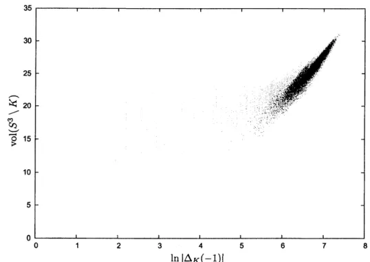
$0$ 1 2 3 4 5 6 $\ln|\Delta_{K}(-1)|$

7

FIGURE 1. Plot of$vol(S^{3}\backslash K)$ against $\ln|\triangle_{K}(-1)|$ for hyperbolic knots $K$

with at most fifteen crossings. 35 30 25 $\hat{/}\aleph_{20}$ $\mathring{C}_{O}\overline{O}15\triangleright$ 10 5 $0$ $0$ 0.5 1 1.5 2 2.5 3 3.5 4 4.5 $\ln(m(\Delta_{K}))$

FIGURE 2. Plot of$vol(S^{3}\backslash K)$ against $\ln(m(\Delta_{K}))$ for hyperbolic knots $K$

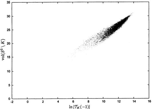
$-2$ $0$ 2 4 6 6

$\ln|\mathcal{T}\kappa(-1)|$

10 12 14

FIGURE

3.

Plot of$vol(S^{3}\backslash K)$ against $\ln|\mathcal{T}_{K}(-1)|$ for hyperbolic knots $K$

with at most fifteen crossings.

0.5 $0$ 0.5 $\{$ 1.5 2 2.5 3 3.5 4

$\ln|\mathcal{T}_{K}(+1)|$

FIGURE 4. Plot of$vol(S^{3}\backslash K)$ against $\ln|\mathcal{T}_{K}(+1)|$ for hyperbolic knots $K$

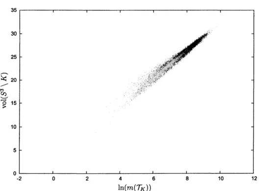
$-2$ $0$ 2 4 6

$\ln(m(\mathcal{T}_{K}))$

8 10

FIGURE 5. Plot of $vol(S^{3}\backslash K)$ against $\ln(m(\mathcal{T}_{K}))$ for hyperbolic knots $K$

with at most fifteen crossings.

35 30 25 $\hat{/}\aleph_{20}$ $n_{O}c_{\overline{O}15}$ $\{0$ 5 $0_{0}$ 0.5 1 1.5 2 2.5 3 $\ln(m(J_{K}))$

FIGURE 6. Plot of $vol(S^{3}\backslash K)$ against $\ln(m(J_{K}))$ for hyperbolic knots $K$ with at most fifteen crossings.

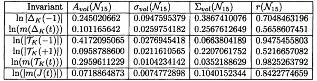
TABLE 2. Calculated data for non-altemating knots with up to fifteen crossings

TABLE 3. Calculated data for all knots with up to fifteen crossings

(1) Note that the average ratio of $m(\triangle_{K}(t))$ to volume is

$0.105675594 \cong\frac{1}{3\pi}$ . 0.995969009.

At

least

a

naive reading of

Section

2 would have suggested that the ratio should

on average

be $\frac{1}{6\pi}$

.

(2) Also note that the average ratio of$m(\mathcal{T}_{K}(t))$ to volume is approximately

$0.296509767 \cong\frac{11}{12\pi}$

.

1.0161959,

our

calculations therefore

are

in line with Conjecture

3.2.

(3) According to the Pearson correlation coefficient the determinant of $K$ correlates

better with the hyperbolic volume than the Mahler

measure

of the Alexander

polynomial, especially for alternatingknots. This also

seems

somewhat surprising considering the discussion of Section 2.

(4) TheMahler

measure

of$\mathcal{T}_{K}(t)$ correlates very highlywith thevolume. The

average

ratioof

0.2965097482

israthermysteriousthough, itis not clear what ‘nice’ number

it corresponds to.

We conclude with

a

list ofopen questions:

(1) Does the Mahler

measure

of knot Floer homology (viewed

as

a multivariable

poly-nomial) correlate

more

with hyperbolic volume than the Mahler

measure

of the

Alexander polynomial?

(2) Does the Mahler

measure

ofKhovanov homology (viewed

as

a

multivariable poly-nomial) correlate

more

with hyperbolic volume than the Mahler

measure

of the Jones polynomial?

(3) Is there any correlation between the Chern-Simons invariant and the arguments

5.

APPENDIX:

THE MAHLER MEASURE

In this appendix we_{will quickly recall the definition and basic} properties oftheMahler

measure

of

a

polynomial. Throughout this section we refer to [Sc95, Section 16] and

[SW04] for details and

references.

Let $p\in \mathbb{C}[t_{1}^{\pm 1}, \ldots, t_{m}^{\pm 1}]$ be a multivariable Laurent polynomial. The Mahler

measure

$m(p)$ ofa

non-zero

polynomial is defined to be

$m(p)= \exp\int_{(S^{1})^{m}}\ln|p(s)|ds$

where we

equip the m-torus $(S^{1})^{d}$ with the Haar

measure.

(Note that the integral is well-defined despite the

zeros

of$p.$)

In the

case

of one-variable polynomials we

can

rewrite the definition as follows: Let $p(t)\in \mathbb{C}[t^{\pm 1}]$ be a polynomial. Then

$m(p(t))= \exp\frac{1}{2\pi}\int_{\theta=0}^{2\pi}\ln|p(e^{i\theta})|d\theta$.

If

$p(t)=ct^{k} \prod_{i=1}^{n}(t-r_{i})$,

then

it

follows from Jensen’s formula

that

$m(p(t))=|c| \cdot\prod_{j=1}^{n}\max(|r_{j}|, 1)$.

REFERENCES

[APS75] M. Atiyah, V. Patodi and I. Singer, Spectml asymmetry andRiemannian geometry II, Math. Proc. Camb. Phil. Soc, 78 (1975), 405-432.

[BV10] N. Bergeron and A. Venkatesh, The asymptotic growth _of torsion homology

_for

arithmetic

groups, Preprint (2010).

[Du99] _{N. Dunfield, An interesting relationship between the Jones polynomial and hyperbolic volume,} unpublished note (1999)

http:$//www$

.

_{math.uiuc. edu}$/\sim$nmd$/prepr$int$s/misc/dylan/$index. html.

[DFJII] N. Dunfield, S. Friedl and N. Jackson, Twisted Alexander polynomials

_of

hyperbolic knots, in

preparation (2011).

[GS91] F. $Gonz\acute{a}lez-Acu\tilde{n}a$ and H. Short, Cyclic bmnched coverings

of

_{knots and homology spheres,}

Revista Math. 4 (1991), 97- 120.

[HTW98] J. Hoste, M. Thistlethwaiteand J. Weeks, The _first 1,701,936 knots, Math. Intell. 20 (1998),

33-48.

[Le09] T. Le, Hyperbolicvolume, Mahler measure, and homology growth, talk at ColumbiaUniversity

(2009),slides available from

http:$//www$

.

_{math.columbia.}$edu/\sim$_{volconf09/notes/leconf.pdf.}

[Le10] T. Le, Homology torsion growth and Mahler measure, Preprint (2010).

[LZ06] W. Li and W. Zhang, An $L^{2}$-Alexander invariant

for

knots, Commun. Contemp. Math. 8

(2006), 167-187,

[L\"u94] W. L\"uck, Approximating $L^{2}$-invariants by their

finite-dimensional analogues, Geom. Funct.

Anal., 4 (1994), 455-481.

[LS99] W. L\"uck and T. Schick, $L^{2}$-torsion

ofhyperbolic _manifolds

_{of finite}

volume, Geom. Funct.

[L\"u02] W. L\"uck, $L^{2}$-invariants: theory and applications to geometry and K-theory, Ergebnisse der

Mathematik und ihrer Grenzgebiete. 3. Folge. A Series of Modern Surveys in Mathematics,

44. Springer-Verlag, Berlin, 2002.

[MP10] P. Menal-Ferrer and J. Porti, Twisted cohomology

for

hyperbolic three manifolds, Preprint (2010).

[Mi66] J. Milnor, Whitehead torsion, Bull. Amer. Math. Soc. 72 (1966), 358-426.

[M\"u09] W. M\"uller, Analytic torsion and cohomology

_of

hyperbolic 3-manifolds, Preprint ofthe

Max-Planck Institute, Bonn (2009).

[M\"u10] W. M\"uller, The asymptotics of the Ray-Singer analytic torsion

_of

hyperbolic S-manifolds, Preprint (2010).

[Po97] J. Porti, Torsion de Reidemeister pour les vanetes hyperboliques, Mem. Amer. Math.Soc. 128

(1997), 612.

[RalO] J. Raimbault, Exponential growth

_of

torsion in abelian coverings, Preprint (2010).

[Ri90] R. Riley, Growth

_of

order

of

homology

_of

cyclic bmnched covers

of

knots, Bull. London Math.

Soc. 22 (1990), 287-297.

[Sc95] K. Schmidt, Dynamical Systems

of

Algebraic $Or\dot{v}gin$, Birkh\"auserVerlag, Basel, 1995.

[Se10] M. H. \S eng\"un, On The Torsion Homology

_of

Non-Arithmetic Hyperbolic Tetmhedml Groups,

Preprint (2010).

[SW02] D. Silver and S. Williams, Mahler measure, links and homology growth, Topology 41 (2002),

979-991.

[SW04] D. Silver and S. Williams, Mahler measure

_of

Alexanderpolynomials, J. London Math. Soc.

(2) 69 (2004), 767-782.

[TuOl] V. Turaev, Intmduction to combinatorialtorsions, Birkh\"auser, Basel, (2001).

MATHEMATISCHES INSTITUT, UNIVERSIT\"AT

zu

K\"oLN, GERMANY

E-mail address: sfriedlQgmail.com

UNIVERSITY OF WARWICK, COVENTRY, UK E-mail address: [email protected]