Stability of traveling waves in curvature flows in the whole plane(Mechanism of temporal and spatial patterns in reaction-diffusion systems)

Stability

of

traveling

waves

in

curvature flows

in

the

whole

plane

東京工業大学大学院情報理工学研究科 奈良光紀(Mitsunori Nara)

Department of Mathematical and Computing Sciences, Tokyo Institute of Tedioloy 1. INTRODUCTION

In this note,

we

study the long time behavior ofsolutions to

a

Cauchy problem of the form

(1) $\frac{u_{t}}{\sqrt{1+u_{x}^{2}}}=\frac{u_{xx}}{(1+u_{x}^{2})^{\frac{\theta}{2}}}+k$, $x\in \mathrm{R},$ $t>0$,

(2) $u(x,0)=u_{0}(x)$, $x\in \mathrm{R}$,

where $k\in \mathrm{R}$ is

a

given

constant.

Especially,

we are

concerned with asymptotic stability

of two types of$\mathrm{t}\mathrm{r}\mathrm{a}\mathrm{v}\mathrm{e}1_{\dot{\mathrm{i}}}\mathrm{g}$

waves:

the traveling lines and the $V$-shaped

flonts.

Our

motivation tostudythisproblem

comes

from the theoryof interfacialphenomena,

which is apart of mathematical science and is concerned with formation and development of

a

“shape” in biological, chemical, and physicalfields. One of the mathematical models that describes the motion ofinterfaces is

a

curvature

_flow.

Let $D(t)$ be

a

moving domain in $\mathrm{R}^{2}$

with

a

smooth boundary $\Gamma(t)=\partial D(t)$

.

Let $\nu$ be

the unit normal vector

on

$\Gamma(t)$ pointing from $D(t)$ to $D(t)^{\mathrm{C}}$

.

We consider an interface

$\Gamma(t)$ governed by

a

curvature

flow with

constant

driving force $k\in$R. Namely,

we

have

(3) $V=-H+k$,

where $V$ and $H$

are

the normal velocity and the curvature of $\Gamma(t)$, respectively. That

is, $V$ is the velocity of $\Gamma(t)$ along $\nu$

,

and $H=\mathrm{d}\mathrm{i}\mathrm{v}\nu$

.

This model appears in several

fields. One of them is the dynamics of interfaces in an excitable media, for example, Belousov-Zhabotinsky reaction $[3, 27]$

.

Equation (3) also

appears

in the dynamics of interfaces in the

Allen-Cahn

equations. See [5] for instance. Moreover it appears in the reaction-diffusionsystems of

a

competition type. See [10].

In this note,

we

deal with the

case

where an initial curve is given by a function $y=$

$u_{0}(x),$$x\in \mathrm{R}$, and

a

moving

curve

is expressed by $y=u(x,t),x\in \mathrm{R},t>0$

.

Under these

assumptions, (3) is rewritten

as

the initial value problem (1) $-(2)$

.

1.1. Traveling

waves

inthe curvature flow. Amoving

curve

$\Gamma(t)$ is called

a

traveling

wave

of (3) with thevelocity $|v|$

,

if$\Gamma(t)$ satisfies

$\Gamma(t)=\Gamma(\mathrm{O})+vt$, $t>0$

for

some vector

$v\in \mathrm{R}^{2}$

.

When _{$k\neq 0$},

a

stationary circle with radius _$1/k$ is

a

traveling

wave

with $|v|=0$

.

Except for this circle and self-crossing ones,

a

traveling

wave

of

$V=-H+k(k\neq 0)$ is

one

ofthe folowing two

cases

$[3, 23]$:

$\bullet \mathrm{k}\neq 0$

(a) Stationary circle (b) Travelingline $(\mathrm{c})$ $\vee$-shaped front

$\bullet$ $\mathrm{k}=0$ (Curve shortening flow)

($\theta$ Expanding

(d) _Grim reaper (e) Stationaryline _{self-similar solution} FIGURE 1. Characteristic

waves

ofthe curvature flow.

(ii) The $V$-shaped front, which is

convex

and is asymptotic to the traveling lines at

infinity.

As is mentioned later, the traveling lines and the$\mathrm{V}$-shaped fronts

can

be represented by

graphical forms under

an

appropriate rotation of coordinates.

On

the

other

hand, $k=0$

means

the

so-called

curve

shortening flow, which is

the

mean

curvature flow in $\mathrm{R}^{2}$

.

In this case,

every

line is

a

stationary

wave,

and there exists

a

traveling

wave

that is$\mathrm{c}\mathrm{a}\mathrm{U}\mathrm{e}\mathrm{d}$ the

Grim

Reaper. Furthermore the

curve

shortening flow has

an

extracting self-similar solution, which is

convex

and is asymptotic to the stationary lines

as

$|x|arrow\infty$

as

in $[9, 18]$

.

Letting $k\in \mathrm{R}$ be

an

arbitrary constant,

we

study asymptotic stability of the traveling (or stationary) lines. Inaddition,

we

consider asymptotic stabilityofthe$\mathrm{V}$-shapedfronts

for $k>0$

.

Especially

we

are

interestedin the large timebehavior of these traveling

waves

for

some

initial perturbations that do not decay as $|x|arrow\infty$

.

1.2. Profiles of the traveling line and the $\mathrm{V}$-shaped front. We

assume

that

a

traveling

wave

in$\mathrm{R}^{2}$

moves

along the $y$-axis without loss of generality. To obtainprofiles

of the traveling lines and the $\mathrm{V}$-shaped fronts,

we

substitute $u(x,t)=U(x)+ct$ to (1),

and obtain

an

ordinary differential equation

(4) $c= \frac{U’’}{1+(U’)^{2}}+k\sqrt{1+(U’)^{2}}$, $x\in \mathrm{R}$.

For any $k\in \mathrm{R}$ and $m\in \mathrm{R}$, traveling lines

are

obtained

as

FIGURE 2. The graph of

a

$\mathrm{V}$-shaped front.

These traveling lines have velocity $k$ in the normal direction and velocity $c$ in the $y-$

direction.

On

the other hand, the $\mathrm{V}$-shaped front is another solution of(4). The exact

represen-tation of

the

profile ofthe$\mathrm{V}$-shaped front $\Phi(x;c, k)$ is written

as

follows.

Proposition 1.1 (Ninomiya and Taniguchi [23]). For

$c>k>0,$

(4) has

a

solution

$\Phi(x;c, k)$ represented by

$x(\theta)=$ $\frac{\theta}{c}+\frac{k}{c\sqrt{c^{2}-k^{2}}}\log|\frac{1+\sqrt{=^{c-k}c+k}\tan_{2}\theta}{1-\sqrt{c+kc-k}\tan_{2}\theta}=|$ ,

$y(\theta)=$ $\frac{1}{c}\log(\frac{2(c^{2}-k^{2})}{c(c\cos\theta-k)})+\frac{\sqrt{c^{2}-k^{2}}}{ck}\arctan(\frac{\sqrt{c^{2}-k^{2}}}{k})$,

for

$\theta\in(-\arctan m, \arctan m)$

.

Here $m=\sqrt{c^{2}-k^{2}}/k$. Moreover $\Phi(x;c, k)$ is strictly

convex

urith

$\Phi_{xx}(x;c, k)>0$, $x\in$ R.

From Proposition 1.1,

we

find that $\Phi(x;c, k)$,

or

$\Phi(x)$ in short, satisfies

(5) $\Phi’,\Phi’’$, and $\Phi’’’$

are

continuous and bounded

on

$\mathrm{R}$,

(6) $\lim_{xarrow-\infty}\Phi(x)=-mx$, $\lim_{xarrow+\infty}\Phi(x)=mx$,

We note that, for each

$c>k>0$

, the problem (1) $-(2)$ has three traveling

waves:

the traveling lines$y=\pm mx+ct,$ $m=\sqrt{c^{2}-k^{2}}/k$, and the$\mathrm{V}$-shapedfront $y=\Phi(x;c, k)+ct$

that

is asymptotic

to

the traveling $1\mathrm{i}\mathrm{n}\mathrm{e}\mathrm{s}\pm mx+ct$

as

$xarrow\pm\infty$.

1.3.

Stability oftraveling

waves.

Tostudy stability ofthe travelingline $y=mx+ct$,

we

consider

a

function$\overline{u}(x,t)=u(x,t)-(mx+ct)$

.

Then

we

have

a

quasi-linearparabolic

equation

$\overline{u}_{t}$ $=$ $\frac{\overline{u}_{xx}}{1+(\overline{u}_{x}+m)^{2}}+k(\sqrt{1+(\overline{u}_{x}+m)^{2}}-\sqrt{1+m^{2}})$

$=(\arctan(\overline{u}_{x}+m))_{x}+k(\sqrt{1+(\overline{u}_{x}+m)^{2}}-\sqrt{1+m^{2}})$ ,

where $c=k\sqrt{1+m^{2}}$

.

Similarly, for the $\mathrm{V}$-shaped front

$\Phi(x;c, k)$,

we

have

$\overline{u}_{t}=(\arctan(\overline{u}_{x}+\Phi’))_{x}+k(\sqrt{1+(\overline{u}_{x}+\Phi’)^{2}}-\sqrt{1+m^{2}})$

.

In these equations,

every

constant,thatis, $\overline{u}(x,t)\equiv(\mathrm{c}\mathrm{o}\mathrm{n}\mathrm{s}\mathrm{t}.)$

,

implies

a

$\mathrm{t}\mathrm{r}\mathrm{a}\mathrm{v}\mathrm{e}1_{\dot{\mathrm{i}}}\mathrm{g}$

wave

with

translationin$y$-direction. Thusevery constant is

a

stationary solution of these equations.

For the Cauchy problem of the heat equation

(8) $h_{t}=h_{xx}$, $x\in \mathrm{R},$ $t>0$,

(9) $h(x,0)=\varphi(x)$, $x\in \mathrm{R}$,

it is well known that every constant is a stationary solution and i8 asymptotically stable in $L^{\infty}(\mathrm{R})$ for spatially decaying initial perturbations. To be

more

precise, a stationary

solution $h(x,t)\equiv\mu$ of (8) $-(9)$ is asymptotically stablein $L^{\infty}(\mathrm{R})$ ifand onlyifthe initial

value $\varphi(x)$ satisfies

$\lim_{Rarrow\infty}\sup_{x\in \mathrm{R}}\frac{1}{2R}|\int_{x-R}^{x+R}\varphi(y)-\mu dy|=0$.

For the proof,

see

[11, 19, 20, 29]. In relation to this criterion, Collet

&Eckmann

[8] showed the example of

an

initial perturbation for which the

constant

solution

of

(8)

-(9) loses the asymptotic stability, where the bounded initial value does not decay but oscillates slower and slower

as

$|x|arrow\infty$

.

Proposition

1.2

(Collet and Eckmann [8]). Let $L_{n}=n!$ and

define

an even

junction

$\varphi^{*}(x)\in C^{\infty}(\mathrm{R})$ that

satisfies

$|\varphi^{*}(x)|\leq 1$

for

$x\in \mathrm{R}$ and

$\varphi^{*}(x)=(-1)^{n}$, $x\in[L_{n}+2^{n}, L_{n+1}-2^{n+1}]$

for

$n\geq 5$

.

Then the solution $h(x, t)$

of

(8) - (9) with $h(x,\mathrm{O})=\varphi^{*}(x)$

satisfies

$\lim\inf h(0,t)=-1tarrow\infty$’ $\lim_{tarrow}\sup_{\infty}h(0,t)=1$

.

In [21],

we

also obtained the following example for thecurvature flow (1) $-(2)$

.

In this example, the initial perturbation looks like $\varphi^{*}(x)$ in Proposition 1.2, that is, it does not

decaybut oscillates slower and slower at infinity.

Example 1.3 (Nara and Taniguchi [21]).

_Define

a

_function

$f(x)$

as

$f(x)=0$

_if

$(2n)^{2}\leq|x|<(2n+1)^{2}$, $f(x)=1$

_if

$(2n+1)^{2}\leq|x|<(2n+2)^{2}$,

for

$n=0,1,2,$$\ldots$

.

Then the solution

of

(1) $-(2)$ with$u_{0}(x)=(\eta*f)(x)$ does not converge

uniformly to the traveling line $u(x, t)=kt+\mu$

_for

any

fixed

$\mu$

.

Here $\eta*is\mathfrak{W}ed\dot{n}chs$

’

mollifier, that is, $\eta(x)\in C_{0}^{\infty}(\mathrm{R}),$ $\eta(x)\geq 0,||\eta||_{L^{1}(\mathrm{R})}=1$, and

$( \eta*f)(x)=\int_{\mathrm{R}}\eta(x-y)f(y)dy$

.

It is also known that the $\mathrm{V}$-shaped front of the Cauchy problem (1) $-(2)$ is not

asymp-totically stable for similar perturbations

as

in [24]. Moreover Po16kSik&Yanagida [28] studiedrelated works

on

a

supercritical semi-linear diffusion equation.

Such counter-examples may causedifficulty in considering asymptotic stabihty of

con-stant

solutions in the Cauchy problem of

a

parabolic PDE with

an

initial perturbation

that does

not

decay

at

infinity.

1.4. Outline ofthis

note.

In

Section

2,

we

consider asymptoticstabilityofthe traveling lines. In Section 3,

we

give

some

examples ofspatialy non-decaying initialperturbations for which traveling lines lose the asymptotic stability. In Section 4,

we

consider the asymptotic stability ofthe $\mathrm{V}$-shaped fronts. Finally in

Section 5 we

show the outline of

proofs.

Our results in this note

for

the traveling lines and the$\mathrm{V}$-shapedfronts

are

based

on

the

discussions in [21] and [22]. We omit most ofproofs. See [21] and [22] for further details.

1.5.

Notation. Inwhat folows, $L^{1}(\mathrm{R}),$ $L^{\infty}(\mathrm{R}),$ $W^{1.\infty}(\mathrm{R})$

,

denote the Lebesgue

or

Sobolev

spaces. For$7\in(0,1),$ $C^{\gamma}(\mathrm{R})$denotes theH\"olderspace, that is, thespaceof functions that

are

bounded and uniformly H\"older continuous with exponent $\gamma$

on

R. $C^{2+\gamma}(\mathrm{R})$

means

the

space

of functions with $u,u’,u”\in C^{\gamma}(\mathrm{R})$

.

For

a

domain $R_{T}=\mathrm{R}\cross[0,T],$ $C^{\gamma,\gamma/2}(R_{T})$

denotes the space of functions that

are

bounded and uniformly H\"older continuous with exponent _{7 and} $\gamma/2$ with respect to $x$ and $t$, respectively

on

$R_{T}$

.

$C^{2\mapsto,1+\gamma/2}(R_{T})$

means

the

space

offunctions with $u,u_{x},u_{xx},u_{t}\in C^{\gamma,\gamma/2}(R_{T})$

.

2.

STABILITY

OF TRAVELING LINES

In this section,

we

show the asymptotic stability of traveling lines$y=mx+ct$ of(1)

-(2). In what follows, let $k\in \mathrm{R}$ and $m\in \mathrm{R}$ be given constants, and put $c=k\sqrt{1+m^{2}}$

.

First

we

considerthe stability with spatially decaying initial perturbations. Nextwe focus on the stability of traveling lines with spatially non-decaying initial perturbations. The key to

our

discussion is the concept of an almostperiodic

_function.

2.1. Stability with spatially decaying perturbations. First

we

give

a

result for the horizontal traveling line $u(x,t)=kt$, that is, the

case

of$m=0$.

Theorem 2.1. Suppose that $\phi\in C^{2+\gamma}(\mathrm{R})$

satisfies

$\lim_{|x|arrow\infty}\phi(x)=0$. Then

for

the

initial value $u_{0}(x)=\phi(x)$, the solution $u(x,t)$ to the Cauchy problem (1) - (2) exists up

to

$t=\infty$

.

Moreover it

satisfies

$\lim_{tarrow\infty}\sup_{x\in \mathrm{R}}|u(x,t)-kt|=0$

.

Especially,

_if

$\phi$ belongs to $C^{2+\gamma}(\mathrm{R})\cap L^{1}(\mathrm{R})$, the solution$u(x, t)$

satisfies

the estimate $\sup_{x\in \mathrm{R}}|u(x,t)-kt|\leq C(1+t)^{-\mathrm{z}}1$, $t>0$,

This result is similar to that for the Cauchy problem

of the

heat equation. By virtue ofthis result,

we

also obtain

a

result for the inclined traveling line $y=mx+ct,$ $m\in \mathrm{R}$

as

follows.

Theorem 2.2. Suppose that $\phi\in C^{2+\gamma}(\mathrm{R})$

satisfies

$\lim_{|x|arrow\infty}\phi(x)=0$. Then

for

the

initial value$u_{0}(x)=mx+\phi(x)$, the solution$u(x,t)$ to the Cauchyproblem (1) $-(2)$

eansts

up to $t=\infty$. Moreover it

satisfies

$\lim_{tarrow\infty}\sup_{x\in \mathrm{R}}|u(x,t)-(mx+ct)|=0$

.

2.2.

Stability with spatially non-decaying initial perturbations. Next

we

show the asymptotic stability with spatially non-decaying initial perturbations. We begin by recallingthe definitionof

an

almost periodic function.

Definition

2.3.

A continuous $fi_{A}nctionf(x)$ : $\mathrm{R}arrow \mathrm{R}$ is called

an

almost periodic

jfunction (in the $\mathit{8}ense$

of

Bohr) if,

for

every$\epsilon>0$, there evists $\ell(\epsilon)>0$ such that,

for

every$p\in \mathrm{R}$,

an

interval $[p,p+\ell(\epsilon)]$ contains at least

one

number$q$ with

(10) $|f(x-q)-f(x)|<\epsilon$

for

all $x\in \mathrm{R}$

.

For any almostperiodic

_function

$f$, there exists

a

mean

$\mathcal{M}\{f\}$

defined

by $\mathcal{M}\{f\}=\lim_{Rarrow\infty}\frac{1}{R}\int_{s}^{\epsilon+R}f(x)dx$,

where the convergence is

_uniform

with respect to $s\in \mathrm{R}$, and the limit is independent

of

$s$

.

By thiv definition,

every

periodic function is

an

almost periodic function.

Moreover

if

$f$ and $g$

are

both ahnost periodic functions, $f(x)+g(x)$ is

an

almost periodic function,

where$\mathcal{M}\{f+g\}=\mathcal{M}\{f\}+\mathcal{M}\{g\}$ holds true. Note that

a

non-periodic function $f(x)=$

$\sin x+\sin\sqrt{2}x$ is

an

almost periodic function with $\mathcal{M}\{f\}=0$

.

For further details,

see

[1, 2, 7] for instance.

Thefollowing result is the central point of

our

discussion for asymptotic stability with spatialy non-decaying initial perturbations. This implies that the almost periodicity of

an

initial perturbation is sufficient for asymptotic stability of traveling lines.

Theorem 2.4. Assume that$\phi\in C^{2\mapsto}(\mathrm{R})$ is

an

almost_$pe$riodic

function.

Then

for

the

initial value$u_{0}(x)=mx+\phi(x)$, the solution$u(x, t)$ to the Cauchy problem (1) $-(2)e$tists up to $t=\infty$

.

Moreover it

satisfies

$\lim_{tarrow\infty}\sup_{x\in \mathrm{R}}|u(x,t)-(mx+ct+\mu)|=0$

for

a constant

$\mu$ with

$\inf_{x\in \mathrm{R}}\phi(x)\leq\mu\leq\sup_{x\in \mathrm{R}}\phi(x)$.

Especially

_for

each $\phi$, the constant

$\mu$ is a nondecreasing

function

of

$k\in \mathrm{R}$ when $m=0$

.

In addition, $\mu=\mathcal{M}\{\phi\}$ holds true when$k=0$

.

We show the outline of the proof of Theorem 2.4 in Section 5. The constant $\mu$ in

Theorem 2.4 may not be determined explicitly if $k\neq 0$

.

Indeed

we

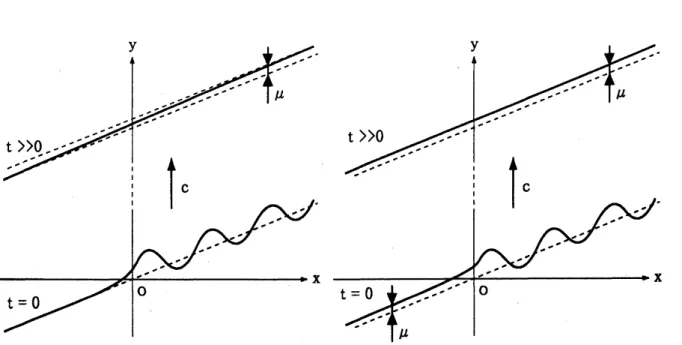
have the following

FIGURE

3.

Stability with

an

almost periodic function

as an

initial perturbation. Remark

2.5.

Generically $\mu\neq \mathcal{M}\{\phi\}$ holds

true

if

$k\neq 0$

.

Indeed,

for

$k>0$ and

$\phi(x)=\sin x$

, we

have

$\mu=\lim_{tarrow\infty}\frac{1}{2\pi}\int_{0}^{2\pi}u(x, t)dx=\frac{1}{2\pi}\int_{0}^{2\pi}\phi(x)dx+\frac{1}{2\pi}\int_{0}^{\infty}\int_{0}^{2\pi}u_{t}(x,t)dxdt$

$= \frac{1}{2\pi}\int_{0}^{\infty}([\arctan(u_{x}+m)]_{0}^{2\pi}+\int_{0}^{2\pi}k(\sqrt{1+(u_{x}+m)^{2}}-\sqrt{1+m^{2}})dx)dt$

$> \frac{1}{2\pi}\int_{0}^{\infty}\int_{0}^{2\pi}k\frac{mu_{x}}{\sqrt{1+m^{2}}}dxdt=\frac{km}{2\pi\sqrt{1+m^{2}}}\int_{0}^{\infty}[u]_{0}^{2\pi}dt=0$

by using the periodic boundary condition at$x=0,2\pi$, and the inequality

$\sqrt{1+(p+m)^{2}}\geq|\frac{mp}{\sqrt{1+m^{2}}}+\sqrt{1+m^{2}}|\geq\frac{mp}{\sqrt{1+m^{2}}}+\sqrt{1+m^{2}}$

for

$p\in \mathrm{R}$

.

Thus

$\mu$

differs from

$\mathcal{M}\{\phi\}=0$ in this

case.

We

can

extend Theorem

2.4

to the

case

where

an

initial perturbation is asymptotic to

an

almost periodic function

as

$|x|arrow\infty$. The following theorem gives. the bounds for

a

perturbation depending only

on

the asymptotic behavior of

a

given initial perturbation

at infinity.

Theorem

2.6.

For

some

_functions

$\phi_{*}(x)$ and$\phi^{*}(x)$ thatbelong to $C^{2+7}(\mathrm{R})$, let$u_{l}(x,t)$

and $u^{*}(x,t)$ be the solutions

of

(1) - (2) with the initial values $mx+\phi_{*}$ and $mx+\phi^{*}$,

respectively. Assume that $u_{*}$ and $u^{*}$

satish

for

some constants

$\mu_{*}$ and$\mu^{*}$

.

Then

for

an

initialperturbation $\phi\in C^{2+7}(\mathrm{R})$ with

$\lim_{xarrow-\infty}(\phi(x)-\phi_{*}(x))=0$, $\lim_{xarrow+\infty}(\phi(x)-\phi^{*}(x))=0$,

the solution $u(x,t)$

of

(1) $-(2)$ with $u_{0}(x)=mx+\phi(x)$ exists up to$t=\infty$

.

Moreover it

satisfies

$\lim_{tarrow\infty}\inf_{x\in \mathrm{R}}(u(x,t)-(mx+ct+\min\{\mu_{*}, \mu^{*}\})=0$,

$\lim_{tarrow\infty}\sup_{x\in \mathrm{B}}(u(x,t)-(mx+ct+\max\{\mu_{*}, \mu^{*}\})=0$

.

This

extends

a

class of imitial values for which the stability is determined. The

following

corollary gives

an

extended sufficient

condition

for

the asymptotic stability of traveling

$1_{\dot{\mathrm{i}}}\mathrm{e}\mathrm{s}$

.

Corollary

2.7. Assume

that $f\in C^{2+\gamma}(\mathrm{R})$ is

an

almostperiodic

fimction.

And $ass\mathrm{u}me$

that $g\in C^{2+\gamma}(\mathrm{R})$

satisfies

$\lim_{|x|arrow\infty^{g(x)}}=0$

.

Then the solution $u(x,t)$ to the Cauchy

problem (1) $-(2)$ with the initial value $u_{0}(x)=mx+f(x)+g(x)$

satisfie8

$\lim_{tarrow\infty}\sup_{x\in \mathrm{R}}|u(x,t)-(mx+ct+\mu)|=0$

for

a constant

$\mu$ that depends only

on

$k,m$, and $f$, and is independent

of

$g$

.

Especially,

$\mu=\mathcal{M}\{f\}$ holds

true

if

$k=0$

.

3.

EXAMPLES FOR ASYMPTOTIC STABILITY OF TRAVELING LINES

In this section

we

show

some

examples and counter-examples for stability oftraveling lines. If

a

given inlitial perturbation $\phi(x)$

on

the traveling line $mx+ct$ is bounded, we

have

$\inf_{x\in \mathrm{R}}\phi(x)\leq u(x,t)-(mx+ct)\leq\sup_{x\in \mathrm{R}}\phi(x)$, $x\in \mathrm{R},$ $t>0$,

by using the comparison principle. This implies that atraveling line is always stable for bounded perturbations. The problem is the asymptoticstability for these perturbations. Example 3.1. The solution $u(x,t)$ to the Cauchy problem (1) - (2) with the initial

value $u_{0}(x)=mx+\tanh x$

satisfies

$\lim_{tarrow\infty}\inf_{x\in \mathrm{R}}(u(x,t)-(mx+ct))=-1$, $\lim_{tarrow\infty}\sup_{x\in \mathrm{R}}(u(x,t)-(mx+ct))=1$.

Though this example is intuitively clear, it is proved rigorously by virtue ofTheorem

2.6.

Namely, $\tanh x$ is asymptotic to $\pm 1$ at infinity, and the solutions with the imitial

value $mx+1$ and mx–l

are

given by$u^{*}(x,t)=mx+ct+1$ and $u_{*}(x,t)=mx+ct-1$,

respectively. Thus Theorem

2.6

gives Example

3.1.

Thenext example shows difficultyof asymptotic stability for $k\neq 0$ compared with $k=0$

.

Example

3.2.

_Define

the initialperturbation $\phi(x)\in C^{2+\gamma}(\mathrm{R})$ to

satish

$\phi(x)=0$

if

$x\in(-\infty, -1]$, $\phi(x)=\sin x$

if

$x\in[1, +\infty)$

.

FIGURE 4. Initial values and the solutions in Example

3.2

and 3.3

Then the solution$u(x,t)$ to the Cauchy problem (1) $-(2)$ with$u_{0}(x)=mx+\phi(x)$

satisfies

$\lim_{tarrow\infty}\sup_{x\in \mathrm{R}}|u(x,t)-mx|=0$

if

$k=0$, $\lim_{tarrow\infty}\inf_{x\in \mathrm{R}}(u(x, t)-(mx+\mathrm{c}t))=0,\lim_{tarrow\infty}\sup_{x\in \mathrm{R}}(u(x, t)-(mx+ct))=\mu$

if

$k>0$

for

a

positive constant $\mu$

.

This example follows from Theorem

2.6

and Remark

2.5.

It is due to the fact that

a

phase shift ofthe limiting traveling line

occurs

if $u_{0}(x)=mx+\sin x$, while it does not

occur

for $\mathrm{u}_{0}(x)=mx$

.

Arranging this example,

we

have the following

one.

Example 3.3.

_Define

the initial perturbation $\phi(x)\in C^{2+\gamma}(\mathrm{R})$ to

satish

$\phi(x)=\mu$

if

$x\in(-\infty, -1]$, $\phi(x)=\sin x$

if

$x\in[1, +\infty)$,

where

$\mu$

is

the

constant

defined

as

in

Remark

2.5.

Then the solution$\mathrm{u}(x,t)$

to

the Cauchy

prvblem (1) - (2) uyith$u_{0}(x)=mx+\phi(x)$

satisfies

$\lim_{tarrow\infty}\sup_{x\in \mathrm{R}}|u(x,t)-(mx+ct+\mu)|=0$

.

Example

3.2

and

3.3

show thepeculiarityof

our

problem due to

a

phaseshift of the lim-itingtraveling $\mathrm{l}\dot{\mathrm{i}}\mathrm{e}$

.

This mechanismis the point ofdiscussionforthe asymptotic stability oftraveling lines, inaddition to Example

1.3

and Proposition

1.2

in the introduction.

4. $\mathrm{V}$-SHAPED

FRONTS

In this section, letting

$c>k>0$

be any

constants

and setting $m=\sqrt{c^{2}-k^{2}}/k>0$,

we

studyasymptoticstabilityof the$\mathrm{V}$-shaped front $\Phi(x;c, k)$, whichis asymptotic

to

the

traveling $1\mathrm{i}\mathrm{n}\mathrm{e}\mathrm{s}\pm mx+ct$

as

$xarrow\pm\infty$

.

First

we

show asymptotic stability of theV-shaped

fronts for

spatiaily decaying initial perturbations. Ninomiya and Taniguchi proved

the

Theorem 4.1 (Ninomiya and Taniguchi [24]). Suppose that $\phi\in C^{2+\gamma}(\mathrm{R})$

satisfies

$\lim_{|x|arrow\infty}\phi(x)=0$

.

Then

for

the initial value $u_{0}(x)=\Phi(x;c, k)+\phi(x)$, the solution

$u(x, t)$ to the Cauchyproblem (1) - (2) exists up to $t=\infty$

.

Moreover it

satisfies

$\lim_{tarrow\infty}\sup_{x\in \mathrm{R}}|u(x, t)-(\Phi(x;c, k)+ct)|=0$

.

This result is proved by constructing

a

supersolutionand

a

subsolution. In this problem, the decay estimate is not obtained yet. Next weshow the result for spatially non-decaying initial perturbations. In this situation, the key to

our

problem is the stability of

two

asymptotic traveling $1\mathrm{i}\mathrm{n}\text{\’{e}}\pm mx+ct$

.

Theorem

4.2.

For

some

hnctions

$\phi_{*}(x)$ and$\phi^{*}(x)$ in$C^{2+\gamma}(\mathrm{R})$, let$u_{*}(x, t)$ and$u^{*}(x,t)$

be the solutions

_of

(1) $-(2)$ uyiththeinitial$values-mx+\phi_{*}(x)$ and$mx+\phi^{*}(x)$, respectively.

Assume that$u_{*}$ and $u^{*}$

satish

$\lim_{tarrow\infty}\sup_{x<0}|u_{*}(x,t)-(-mx+ct+\mu_{*})|=0,\lim_{tarrow\infty}\sup_{x>0}|u^{*}(x,t)-(mx+ct+\mu^{*})|=0$

for

some constants

$\mu_{*}$ and$\mu^{*}$

.

Then

for

an

initialperturbation $\phi\in C^{2+\gamma}(\mathrm{R})$ with

$\lim_{xarrow-\infty}(\phi(x)-\phi_{*}(x))=0$, $\lim_{xarrow+\infty}(\phi(x)-\phi^{*}(x))=0$,

the solution$u(x,t)$

of

(1) - (2) unth the initial value $u_{0}(x)=\Phi(x;c, k)+\phi(x)$ exis$ts$ up to

$t=\infty$

.

Moreover

it

satisfies

$‘ \lim_{arrow\infty}\sup_{x\in \mathrm{R}}|u(x,t)-[\Phi(x-\frac{\mu_{*}-\mu^{*}}{2m}jc,$$k)+ct+ \frac{\mu_{*}+\mu^{*}}{2}]|=0$

.

Thus the asymptotic stability of the traveling lines $y=\pm mx+ct$ for the initial per-turbations $\phi_{*}$ and $\phi^{*}$ gives the asymptotic stability of the $\mathrm{V}$-shaped front _{$\Phi(x;c, k)$}

.

The

shift ofthe$\mathrm{V}$-shaped front is generically observed in the

case

where initialperturbations

donot decayatinfinity. Combining Theorem

4.2

with Theorem2.4,

we

obtainacorollary that givesconcrete suflicient condition for the asymptotic stability of the$\mathrm{V}$-shaped front.

Corollary 4.3. Assume that$\phi_{*},$ $\phi^{*}(x)\in C^{2+\gamma}(\mathrm{R})$

are

both almost periodic

functions

in

the

sense

_of

Bohr, and let$u_{*}(x,t)$ and$u^{*}(x, t)$ be the solutions

of

(1) -(2) with the initial

$values-mx+\phi_{*}(x)$ and$mx+\phi^{*}(x)$

,

respectiv$\mathrm{e}ly$

.

Then $u_{*}$ and $u^{*}$ exist up

to

$t=+\infty$

,

and satisfy

$\lim_{tarrow\infty}\sup_{x\in \mathrm{R}}|u_{*}(x,t)-(-mx+ct+\mu_{*})|=0$, $\lim_{tarrow\infty}\sup_{x\in \mathrm{R}}|u^{*}(x,t)-(mx+ct+\mu^{*})|=0$

for

some

constants

$\mu_{*}$ and $\mu^{*}$ with

$\inf_{x\in \mathrm{R}}\phi_{*}(x)\leq\mu_{*}\leq\sup_{x\in \mathrm{R}}\phi_{*}(x)$, $\inf_{x\in \mathrm{R}}\phi^{*}(x)\leq\mu^{*}\leq\sup_{x\in \mathrm{R}}\phi^{*}(x)$

.

Moreover

_for

an

initialperturbation $\phi\in C^{2+\gamma}(\mathrm{R})$ with

$\lim_{xarrow-\infty}(\phi(x)-\phi_{*}(x))=0$, $\lim_{xarrow+\infty}(\phi(x)-\phi^{*}(x))=0$,

the solution $u(x,t)$

of

(1) - (2) unth the initial value $u_{0}(x)=\Phi(x;c, k)+\phi(x)$

satisfies

$\lim_{tarrow\infty}\sup_{x\in \mathrm{R}}|u(x, t)-[\Phi(x-\frac{\mu_{*}-\mu^{*}}{2m};$ _$c,$$k)+ct+ \frac{\mu_{*}+\mu^{l}}{2}]|=0$

.

Bythisresult,

a

$\mathrm{V}$-shapedfront with the initialperturbation$\sin x+\sin\sqrt{2}x$is

asymptot-ically stable since this perturbation is an almost periodic function. Moreover aV-shaped front with an smoothinitial perturbation $\phi(x)$ with

$\phi(x)=\{$

$\sin x$, $x\in[0, \infty)$,

$0$, $x\in(-\infty, -1]$,

is

also asymptotically

stable.

This is

clear

by letting $\phi_{*}(x)\equiv 0$

and

$\phi^{*}(x)=\sin x$ in

Corollary

4.3.

This makes sharp

contrast

with Example

3.2

for the traveling lines. 5. PROOF OF THEOREM 2.4

In this section,

we

show the main part of the proofof Theorem 2.4. In what folows,

let $k\in \mathrm{R}$

and

$m\in \mathrm{R}$ be given constants, and put $c=k\sqrt{1+m^{2}}$

.

As

is mentioned in

the introduction,

we

consider the function$\overline{u}(x, t)=u(x, t)-(mx+ct)$ instead

of

$u(x,t)$ in order to analyze the large time behavior ofperturbed traveling lines. Here

we

denote

$\overline{u}(x, t)$ by $u(x, t)$ for simplicity. Then

we

have

(11) $u_{t}=(\arctan(u_{x}+m))_{x}+k(\sqrt{1+(u_{x}+m)^{2}}-\sqrt{1+m^{2}}),$ $x\in \mathrm{R},$ $t>0$,

(12) $u(x, \mathrm{O})=\phi(x)$, $x\in$ R.

It

suffices to

prove the results forthis problem instead of the originalproblem (1) $-(2)$

.

First we show the global existence and some estimates for solutions of (11) - (12). The

following proposition plays important roles in the proof.

Proposition 5.1. Assume that $\phi\in C^{2+\gamma}(\mathrm{R})$

.

Then there exists

a

classical solution

$u(x, t)$ to the Cauchy prvblem (11) -(12) that belongs to $C^{2+\gamma,1+\gamma/2}(R_{T}),$ $R_{T}=\mathrm{R}\cross[0, T]$

for

any$T>0$

.

It

_satisfies

the following estimates

$\sup_{x\in \mathrm{R},t>0}|u(x,t)|\leq||\phi||_{L(\mathrm{R})}\infty,\sup_{x\in \mathrm{R},t>0}|u_{x}(x,t)+m|\leq||\phi’+m||_{L(\mathrm{R})}\infty$,

$\sup_{x\in \mathrm{R},t>0}|u_{xx}(x, t)|\leq C$, $\sup_{x\in \mathrm{R},t>0}|u_{t}(x,t)|\leq C$

.

Here $C$ is

a

constant depending only

on

_{$k,$ $m$}, and $||\phi’||_{W^{1,\infty}(\mathrm{R})}$

.

Remark5.2. Existence

_of

global solutionsto the problem(1) $-(2)$ is aloeady obtainedin

[6] and [23]. Chou&Kwong [6] proved it

_for

a

smooth initial value utthoutthe restriction

of

growth order. Ninomiya&Taniguchi [23] also showed that,

_for

an

initial value $u_{0}(x)=$

$\Phi(x;\mathrm{c}, k)+\phi(x),$$\emptyset\in BC^{1}$, the solution $u(x,t)$

of

(1) - (2) enists globally in time and

satisfies

$u(x,t)-(\Phi(x;c, k)+ct)\in BC^{1}$

for

each $t>0$,

where $BC^{1}=C^{1}(\mathrm{R})\cap W^{1,\infty}(\mathrm{R})$

.

In Proposition 5.1,

we

established the global enistence

of

solutions with

more

detailed estimates

_of

solutions, which

are

suitable and essential

_for

our

later discussions.

In whatfollows,

we

always

assume

that

an

initialvalue

or an

initial perturbationbelongs to$C^{2+\gamma}(\mathrm{R})$

even

ifitisnot mentioned specifically. Here$7\in(0,1)$ is

an

arbitrary

constant.

Lemma 5.3. Assume $k\leq 0$

.

Let$M>0,$ $s>0,$ $T>0$, and $L>0$ be given

constants.

Let$u(x,t)$ be the solution to the Cauchyproblem (11) - (12) with

(13) $||\phi’||_{L(\mathrm{R})}\infty\leq M$,

$\sup_{x\in \mathrm{R}}\phi(x)\leq s$,

(14) $u(a, t)\leq 0$ and $u(b, t)\leq 0$

for

$0\leq t\leq T$

for

a,$b\in \mathrm{R}$ with $a<b$ and $b-a\leq L$

.

Then there exists

a

positive constant $\lambda$ depending

only

on

$M,$ $s,$ $T$ and $L$ with

(15) $\max_{a\leq x\leq b}u(x,T)\leq s-\lambda$

,

where A depends continu$\mathit{0}$usly on$s\in(\mathrm{O}, +\infty)$

for

any

fixed

$M,T$ and$L$.

Next

we

show

a

simple lemma and provide

an

important property of the solution of (11) - (12) with

an

almost periodic function as an initial value. Roughly speaking, for

each $t>0$_{, such}

a

solution has the

same

almost periodicity

as

that of the initial value. Lemma 5.4. Suppose that$\phi(x)$ is

an

almost periodic

function

that

satisfies

(10)

as

in

Definition

2.3

with$\ell(\epsilon)$

.

Let$u(x,t)$ be the solution

of

(11) -(12). Then,

for

evefy$p\in \mathrm{R}$,

an

interval $[p,p+\ell(\epsilon)]$ contains

at

least

one

number $q$ with

$|u(x-q, t)-u(x, t)|<\epsilon$

for

$x\in \mathrm{R},$ $t>0$

.

Now

we

prove the following result, which implies the asymptotic stability of traveling lines for

an

almost periodic function

as an

imitial perturbation. The proof is done by deriving

a

contradiction.

Proposition

5.5.

Suppos$\mathrm{e}$ that $\phi(x)$ is

an

almost periodic

function.

Then the solution

$u(x,t)$

of

(11) -(12)

satisfies

(16) $\lim_{tarrow\infty}\sup_{x\in \mathrm{B}}|u(x,t)-\mu|=0$

for

a constant

$\mu$ that

satisfies

(17) $\inf_{x\in \mathrm{R}}\phi(x)\leq\mu\leq\sup_{x\in \mathrm{R}}\phi(x)$

.

Proof.

Since

all

constants

are

stationary solutions of(11)-(12), the

functions

$U^{+}(t)$ and $U^{-}(t)$ defined by

$U^{+}(t)= \sup_{x\in \mathrm{R}}u(x,t)$, $U^{-}(t)= \inf_{x\in \mathrm{R}}u(x,t)$

are

nonincreasing and nondecreasing, respectively by virtue of the comparison principle. The constants $U^{*}= \lim_{tarrow\infty}U^{+}(t)$ and $U_{*}= \lim_{tarrow\infty}U^{-}(t)$ exist. Now

we

define _$\mu=$

$(U^{*}+U_{*})/2$ and $\delta=(U^{*}-U_{*})/2$

.

Then $\mu$ satisfies (17) because

we

have $U^{-}(0)\leq U$

.

$\leq$

$\mu\leq U^{*}\leq U^{+}(0)$ by the definition.

Since$u(x,t)-\mu$alsosatisfies(11)-(12),

we

may

assume

$\mu=0$withoutlossofgenerality.

Moreover

we

may

assume

$k\leq 0$, since the

case

of$k\geq 0$ is reduced to the

case

of $k\leq 0$

by $\mathrm{c}\mathrm{o}\mathrm{n}\mathrm{s}\mathrm{i}\mathrm{d}\mathrm{e}\mathrm{r}\mathrm{i}\mathrm{n}\mathrm{g}-u(-x,t)$ , which also satisfies (11)-(12).

It suffices to show $\delta=0$

.

In what follows,

we

derive

a

contradiction by assuming

$\delta>0$

.

Suppose that $\phi$ satisfies (10)

as

in Definition

2.3

with $\ell(\epsilon)$

.

We define

a constant

Let $t_{0}>0$ and $x_{0}\in \mathrm{R}$ be arbitrarily fixed. Then we have some points $a\in[x_{0}-L-$

$1,$_{$x_{0}-1]$} and $b\in[x_{0}+1, x_{0}+L+1]$ with

(18) $u(a,t_{0})<- \frac{\delta}{4}$ and $u(b,t_{0})<- \frac{\delta}{4}$.

Indeed, by the definition of $\delta$,

we

can

take

some

point _{$x_{*}\in \mathrm{R}$} with$u(x_{*},t_{0})<-\delta/2$

.

By

virtue of Lemma 5.4, the interval $[x_{*}-x_{0}+1, x_{*}-x_{0}+1+L]$ contains

a

number $q$with $|u(x_{*}-q,t_{0})-u(x_{*}, t_{0})|< \frac{\delta}{4}$

.

Setting $a=x_{*}-q\backslash$’

we

have $a\in[x_{0}-L-1,x_{0}-1]$ and $u(a,t_{0})<u(x_{*}, t_{0})+ \frac{\delta}{4}<-\frac{\delta}{4}$,

whichis thefirst inequality of(18). Similarly

we can

take

a

number$b\in[x_{0}+1, x_{0}+L+1]$

for the second inequality of(18).

Now

we

use

theuniform bound for $|u_{t}|$ obtained byProposition

5.1.

Using thisestimate,

we

obtain

$u(a,t)\leq 0$ and $u(b, t)\leq 0$ for $t_{0}\leq t\leq t_{0}+T$

for

some

positive

constant

$T$ depending only

on

$\phi$ and $\delta$

.

Here

we

shall find

a

positive-valued function $\lambda(s)$ for $s>0$ with

$u(x_{0},t_{0}+T)\leq U^{+}(t_{0})-\lambda(U^{+}(t_{0}))$ .

Using Lemma5.3,

we can

choose $\lambda(\cdot)$ so that $\lambda\in C(\mathrm{O}, +\infty)$ and that it depends only

on

$||\phi’||_{L(\mathrm{B})}\infty,$ $T$ and $2(L+1)$

.

If $U^{+}(t_{0})\geq\delta/2$,

we

get

$u(x_{0},t_{0}+T)\leq U^{+}(t_{0})-\lambda(U^{+}(t_{0}))\leq U^{+}(to)$ $-\lambda_{0}$

.

Here

a

constant

$\lambda_{0}$ is

defined

by

$\lambda_{0}=\min_{\epsilon\in[\delta/2,U^{+}(t\mathrm{o})]}\lambda(s)$.

Notethat $\lambda_{0}$ is wel defined and ispositive. Since$x_{0}\in \mathrm{R}$is arbitrary and$\lambda_{0}$is independent

of$x_{0}$,

we

obtain $U^{+}(t_{0}+T)\leq U^{+}(t_{0})-\lambda_{0}$.

If$U^{+}(t_{0})-\lambda_{0}\geq\delta/2$, the

same

argument

can

be carried out at $t=t_{0}+T$

.

Namely, for

any fixed $x_{0}\in \mathrm{R}$, we have

$u(x_{0},t_{0}+2T)\leq U^{+}(t_{0})-\lambda_{0}-\lambda(U^{+}(t_{0})-\lambda_{0})\leq U^{+}(t_{0})-2\lambda_{0}$

.

Consequently,

we

find that $U^{+}(t_{0}+nT)<\delta/2$for

some

large $n$

.

It folows that $U^{*}<\delta/2$

because$U^{+}(t)$ is

a

nonincreasing. This contradicts the definition of$\delta$

.

Thus $\delta=0$follows,

and the proofofProposition

5.5

is completed.

Remark 5.6. In the

case

_of

$m=0$, that is, in the

case

_of

traveling line $u(x,t)=kt$,

the

constant

$\mu i\mathit{8}$

a

nondecreasing

function of

$k\in \mathrm{R}$

for

each $\phi$

.

For any

fixed

$\phi$

,

let

$u_{1}(x, t)$ and$u_{2}(x, t)$ be the solutions to the problem (11) -(12) uyith $m=0$

for

$k=k_{1}$ and

$k=k_{2}$, respectively. Then there exist

constants

$\mu_{1}$ and$\mu_{2}$ with

It

_suffice

to show$\mu_{1}\geq\mu_{2}$

if

$k_{1}\geq k_{2}$.

If

$k_{1}\geq k_{2}$, we have

$0=$ $(u_{1})_{t}-(\arctan(u_{1})_{x})_{x}-k_{1}(\sqrt{1+(u_{1})_{x}^{2}}-1)$

$\leq$ $(u_{1})_{t}-(\arctan(u_{1})_{x})_{x}-k_{2}(\sqrt{1+(u_{1})_{x}^{2}}-1)$,

which implies that $u_{1}$ is

a

supersolution

of

(11) - (12) with $m=0$ and $k=k_{2}$

.

Thus

$u_{1}(x, t)\geq u_{2}(x, t)$ holds true, and hence $\mu_{1}\geq\mu_{2}$

follows.

Remark

5.7.

In the

case

_of

$k=0$

,

_that is, in the

case

_of

the stationary line $u(x,t)=$

$mx$ in the

curve

shortening flow, $\mu=\mathcal{M}\{\phi\}$ holds

true.

Indeed,

for

any

fixed

$t>0$,

we

have

$\frac{1}{R}|\int_{0}^{R}(u(x,t)-\phi(x))dx|=\frac{1}{R}|\int_{0}^{R}(\int_{0}^{t}u_{t}(x, s)ds)dx|$

$= \frac{1}{R}|\int_{0}^{R}(\int_{0}^{t}(\arctan(u_{x}+m))_{x}ds)dx|\leq\frac{1}{R}\int_{0}^{t}|[\arctan(u_{x}+m)]_{0}^{R}|ds\leq\frac{\pi t}{R}$

.

Therefore

we obtain $| \mathcal{M}\{u\}(t)-\mathcal{M}\{\phi\}|\leq\lim_{Rarrow\infty^{\pi t}}/R=0$

.

It

follows

that $U^{-}(t)\leq \mathcal{M}\{u\}(t)\equiv \mathcal{M}\{\phi\}\leq U^{+}(t)$, $t>0$,

and

hence

$U_{*}=\mathcal{M}\{\phi\}=U^{*}$ in the limit$tarrow\infty$

.

Proof of

Theorem

_2.4.

Theorem

2.4

followsdirectlyfromProposition 5.1, Proposition 5.5,

Remark 5.6, and Remark

5.7.

REFERENCES

[1] A.S.Besicovitch, Almostperiodic ftinctions, DoverPublications, Inc., NewYork, 1955.

[2] H.Bohr, Almostperiodic fimctions, Chelsea, New York, NY, 1951.

[3] P.K.Brazhnik, Exact solutions

_for

the kinematic model

_of

autowaves in two-dimensional excitable

media, Physica D94 (1996), 205-220.

[4] Y.-G. Chen, Y. Giga and S. Goto, Uniqueness and eststence

_of

viscosity solu-tions

_of

generalized

mean cumatufe

_flow

equations, J. Differential Geom. 33 (1991), 749-786.

[5] X.Chen, Generation and propagation

_of

int

_{erfaces for}

_{reaction-diffusion}

equations, J. Differential

Equations96 (1992), 116-141.

[6] K.-S.Chou and Y.-C.Kwong, On quasilinear parabolic equations which admit global solutions

_for

initial datawith unrestricted growth, Calc. Var. PartialDifferentialEquations 12 (2001), 281-315.

[7] C.Corduneanu, Almost periodicfimctions, 2nd Englishedition, Chelsea, NewYork, NY, 1989.

[8] P.Collet and J.-P.Eckmann, Space-time behaviourin problems

_of

hydfvdynamic type: a case study,

Nonlinearity 5 (1992), 1265-1302.

[9] K.Ecker and G.Huisken, Mean curvature evolution

_of

entire graphs, Ann. of Math. 130 (1989),

453-471.

[10] S.-I.Ei and E.Yanagida, Dynamics

_{of interfaces}

in $competition- diffi_{l}sion$ systems, SIAM J. Appl. Math. 54 (1994), 1355-1373.

[11] S.D.Eidel’man, Parabolicsystems, North-Holland, Amsterdam-London; Wolters-Noordhoff,

Gronin-gen, 1969.

[12] L.C. Evansand J.Spruck, Motion

_of

levelsets bymean curvature, J. DifferentialGeom. 33 (1991),

635-681.

[13] A.Friedman, Partial

_differential

equations

_of

parabolic type, Prentice-Hall, Englewood Cliffs, NJ,

1964.

[14] M.Gageand R.Hamilton, The shrinking

_of

convexplane curves by the heat equation, J. Differential Geom. 23 (1986), 69-96.

[15] M.Grayson, The heat equation shrinks embeddedplane curves to points, J. Differential Geom. 26

[16] F.Hamel, R.Monneau and J.-M.Roquejoffre, Enistence and qualitative properties

_of

multi-dimensional conical bistable fronts, preprint.

[17] G.Huisken, Flow bymean curvature

_of

convex

_surface

into surface, J. DifferentialGeom. 20 (1984),

237-266.

[18] N.Ishimura, Curvature evolution

_of

plane curves with prescnbedopeningangle, Bull. Austral. Math.

Soc. 52 (1995), 287-296.

[19] S.Kamenomostskaya, On stabilization

_of

solution

_of

the Cauchy problem

_for

parabolic equations,

Proceedings of theRoyal Societyof Edinburgh, 76A, (1976),43-53.

[20] V.P.Mihailov,Onstabilization

_of

the solution

_of

the Cauchyproblem

_for

the heat conductionequation,

Soviet Math. Dokl., 11 (1970), 34-37.

[21] M.Naraand M.Taniguchi, Stability _ofatravelingwave in cunJatun

_{flows for}

spatially non-decaying perturbations, Discrete and ContinuousDynamical Systems, 14 (2006), 203-220.

[22] M.Nara and M.Taniguchi, Convergence to $V$-shaped

fronts

in curvature

flows for

spatially

non-decaying perturbations, to appearin Discrete and ContinuousDynamical Systems.

[23] H.NinomiyaandM.kniguchi, $\pi avel:ng$curved

fronts

of

amean curvature

flow

urthconstantdriving

force, Free boundary problems: theory and applications, I, Math. Sci. Appl., GAKUTO Internat. Ser. 13 (2000), 206-221.

[24] H.Ninomiya and M.Thniguchi, Stability

_of

traveling curved

_fronts

in a curvature

_flow

utth driving

forne, Methods Appl. Anal. 8 (2001), 429-450.

[25] H.Ninomiyaand M. aniguchi, $E\dot{n}sten\alpha$ and global stability

of

traveling curved$fivnt\epsilon$ in the

Allen-Cahn equations, J. DifferentialEquations,213 (2005), 204-233.

[26] O.A.$\mathrm{L}\mathrm{a}\mathrm{d}ffi\mathrm{n}\epsilon \mathrm{b}\mathrm{j}\mathrm{a}$, V.A.Solonnikov and N.N.Ural’ceva, Linear and Quasilinear Equations

of

Para-bolic IW, Translations of MathematicalMonograph 23,Amer. Math. Soc.,Providence, RI, 1968.

[27] $\mathrm{V}.\mathrm{P}\acute{\mathrm{e}}\mathrm{r}\alpha- \mathrm{M}\mathrm{u}\overline{\mathrm{n}}\mathrm{u}\mathrm{z}\mathrm{u}\mathrm{r}\mathrm{i}$, M.G\’omez-Gesteira, A.P.Munuzuri, V.A.Davydov and V.P\’erez-Villar, V-shaped

stable $non\dot{\varphi}ml$pattems, PhysicalReview E51-2 (1995), 845-847.

[28] P.PolUik and E.Yanagida, Nonstabuiring solutions andgrow-up set_for a supercritical semilinear

diffiwion

equation, Differential IntegralEquations 17 (2004),535-548.

[29] V.D.RepnikovandS.D.Eidel’man, A new prvof

_of

the theoremon the stabilizauon

_of

the solution

of