東北大学機関リポジトリTOUR

Three essays on large-scale public investments

and regional poverty, productivity and

agglomeration in Japan

著者

SUGASAWA TAKERU

学位授与機関

Tohoku University

学位授与番号

11301甲第18408号

Three essays on large-scale public investments and regional

poverty, productivity and agglomeration in Japan

(公共政策が地域経済の貧困、⽣産性、経済集積に及ぼす影響に関する研究)

Takeru Sugasawa

Acknowledgement

First, I am truly grateful to Kentaro Nakajima for his unique advice. His warm encouragement has supported my work. Many facets of this doctoral dissertation were shaped by his useful comments. I also sincerely thank my advisor, Akira Hibiki. His ongoing support greatly help me complete this dissertation.

Further, I would like to thank Lee Huey-Lin for her insightful comments. I am also grateful to have able to participate in the Japanese Economic Association Meeting, the Applied Regional Science Conference, and the International Conference at National Chengchi University.

In addition, I express my appreciation to my laboratory colleagues. Discussions with Yuta Kuroda, Kai Nomura and Takaki Sato contributed to my studies.

Contents

Chapter 1 Introduction

... 1

Chapter 2 Accessibility to the nearest urban metropolitan area and rural poverty in Japan

. 3

Chapter 3 Impacts of constructing flood control dams on industrial investments in downstream regions in the case of Shiga Prefecture

... 30

3.1. Introduction ... 30

3.2. Previous Study ... 31

3.3. Shiga Prefecture and Flood Control Dams ... 32

3.3.1. Shiga Prefecture and Lake Biwa ... 32

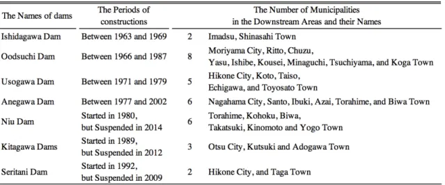
3.3.2. The flood control dams in Shiga Prefecture ... 36

3.4. Empirical Strategy and Data ... 41

3.4.1. Empirical strategy ... 41

3.4.2. Data ... 42

3.5. Results ... 43

3.6. Conclusion ... 57

Chapter 4 Impacts of large-scale developments of water resources on industry of downstream regions in the case of the LBCD project in Japan

... 59

4.1. Introduction ... 59

4.2. The Lake Biwa Comprehensive Development Project ... 61

4.3.1. Estimation models ... 63

4.3.2. Data ... 63

4.3.3. Propensity score matching method... 65

4.4. The Results ... 66

4.5. Conclusion ... 74

List of Figures

Figure 2.1. Routes of the Tsukuba Express and Joban Line………16

Figure 2.2. Regions of the Ibaraki Prefecture and Route of the Tsukuba Express………17

Figure 2.3. Transitions of the Share of Commuters Classified by Commuting Places………28

Figure 3.1. Location of Shiga Prefecture and Lake Biwa………33

Figure 3.2. The Number of Floods in each Municipality between 1895 and 2013………35

Figure 3.3. Map of Flood Control Dams and their Downstream Areas in Shiga Prefecture………38

Figure 3.4. Growth of the Number of Plants (1980=1)………40

Figure 3.5. Location and Establishment Periods of Industrial Parks in Shiga Prefecture………41

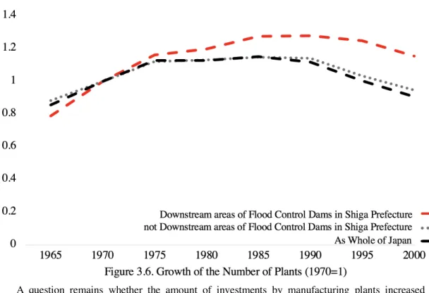
Figure 3.6. Growth of the Number of Plants (1970=1)………51

Figure 4.1. The Map of Prefectures in Kinki Region, Lake Biwa, and Yodo River………62

Figure 4.2. The Map of the Yodo River Water Supply Area………64

Figure 4.3. Location of the Dams Constructed between 1995 and 2005………70

List of Tables

Table 2.1. The Number and Share of Households Discontinuing PA in Japan………10

Table 2.2. Summary Statistics………12

Table 2.3. Results of the Cross-Sectional Analysis………14

Table 2.4. Summary Statistics of the Panel Analysis………20

Table 2.5. Results of the Panel Analysis………21

Table 2.6. Distribution of Household Income in Ibaraki Prefecture………23

Table 2.7. Results of Opening TX on the Number of Households Divided by their Income………26

Table 2.8. The Number and Share of Households Divided by Monthly Rent and Duration of Residence in 2013………27

Table 3.1. Flood Damage by Year in Shiga Prefecture………36

Table 3.2. Construction of Flood Control Dams between 1965 and 2000………37

Table 3.3. Summary Statistics………43

Table 3.4. Results of the Event Study………44

Table 3.5. The Number and Share of Manufacturing Plants Categorized by Manufacturing Types and Amounts of Capital………45

Table 3.6. Summary Statistics of the Number of Plants Classified by the Manufacturing Categories……47

Table 3.7. Results of the Event Study using Samples Classified by Manufacturing Categories…………49

Table 3.8. Results of the Event Study focusing on the Amounts of Investment………53

Table 3.9. Statistical Statuses of the Commerce Industry in each Dam's Downstream Area………54

Table 3.10. Spillover Effects of Flood Risk Reduction on the Number of Commerce Shops………57

Table 4.1. Summary Statistics of Matched and not-Matched Samples………66

Table 4.2. Impacts of the LBCD project on Agricultural and Fishery Industries in Downstream Areas…68 Table 4.3. Results of the Placebo Test………69

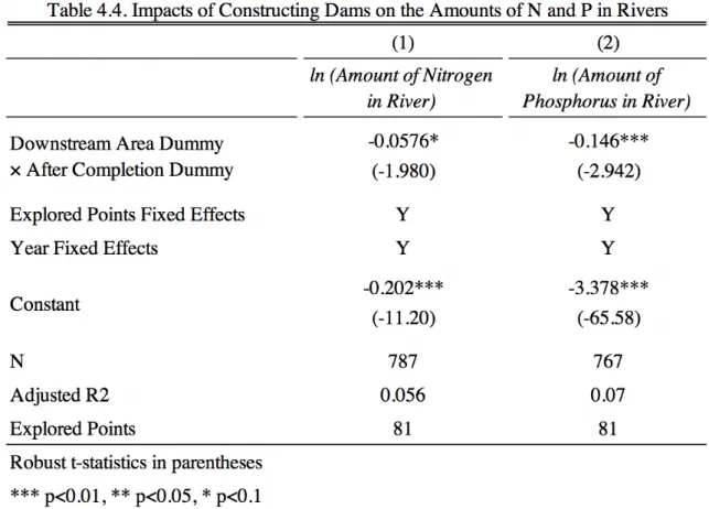
Table 4.4. Impacts of Constructing Dams on the Amounts of N and P in Rivers………71

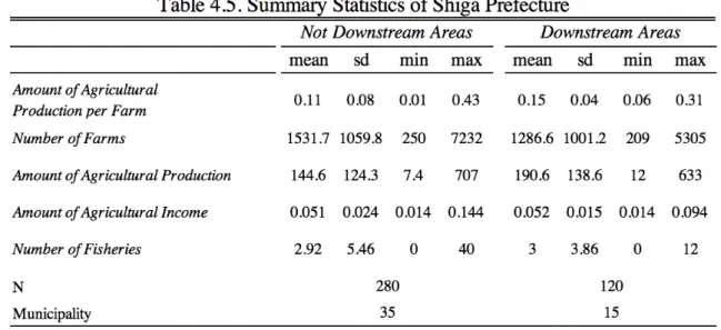
Table 4.5. Summary Statistics of Shiga Prefecture………73

Chapter 1

Introduction

Public investment is one of the most important ways to activate economic activities, and thus, a large volume of funds is invested by national and regional governments. For instance, the Japanese national government invested approximately 27.8 trillion yen in 2017, representing approximately 5.2% of its real GDP. To find more efficient means of public investment, many studies have investigated the impacts of public works (Kline and Moretti: 2013, Busso, Gregory and Kline: 2013).

As an important means to stimulate economic activities, industrial agglomeration has been examined by urban economists (Fujita, Krugman and Venables: 2001, Fujita and Thisse: 2013). Industrial agglomeration activates a region’s economic activities through rich labor markets, low transportation costs of inputs and outputs, and knowledge spillovers (Marshall: 1920, Rosenthal and Strange: 2004). In addition, positive effects of economic agglomeration are known to spill over to areas in close proximity to urban metropolitan areas (Feldman: 1999). Since many developed countries are facing serious declines in population, it is important to investigate ways to extend economic agglomeration or to expand the range of positive spillover effects.

From the abovementioned background, we focus on public investments that have affected the scale of regional economic agglomeration or that have expanded the range of spillover effects of economic agglomeration. Our empirical analyses suggest that public investments improving accessibility to areas in close proximity to urban metropolitan areas can expand the range of positive spillover effects of economic agglomeration. In addition, we find that governments can expand economic agglomeration and stimulate regional economic activities through public investments that mitigate disaster risks. However, we also find that public works aimed at decreasing disaster risks could have negative side effects in limiting the agglomeration of specific industries.

This dissertation covers three independent empirical studies based on Japanese municipal-level data. In chapter 2 we examine the effects of accessibility to the nearest urban metropolitan area on rural poverty. The magnitude of positive agglomeration spillover effects decreases with distance from urban metropolitan areas, and regional economic performance can decrease with distance from economic agglomerations (Rosenthal and Strange :2003, 2006). We conduct nationwide cross-sectional analyses and find significant increases in regional poverty rates with time distance from the nearest urban metropolitan area. In addition, the study focuses on the establishment of a new commuting train, Tsukuba Express (TX), connecting Tokyo to Ibaraki prefecture, a suburban area of Tokyo. We conduct municipal-level panel

analyses, and our results suggest the opening of TX reduced rural poverty rates in the surrounding areas but that such effects could only be observed after 6–10 years. Therefore, regional policy makers may need to ensure that transportation investments that improve interregional accessibility do not affect regional economic performance for several years.

In chapter 3 we investigate the impacts of flood control dam construction on the location decisions of industries operating in downstream areas. It may be that disaster risks prevent regions from developing by decreasing incentives to invest. To analyze these points, we focus on four flood control dams and on 50 municipalities in Shiga prefecture, a suburban area of middle-western Honshu (Japan’s main island), between 1965 and 2000. We conduct event study analyses and find that flood control dam construction significantly increased the number of manufacturing plants of industries requiring a large amount of physical capital in downstream areas. We note that since physical capital only slowly recovers establishment costs, manufacturing categories strongly dependent on physical capital would sensitively react to a reduction of flood risk. We also find that the number of commerce stores increased in areas downstream from the dams. However, the effects took more than 10 years to be observed after the completion of flood control dams. We conclude that the commerce industry witnessed positive effects only after increases in the number of manufacturing plants in operation because the commerce industry was affected by decreases in flood risks through increases in manufacturing plant demands for materials or tools for production activities.

In chapter 4 we analyze effects on primary industries using water resources from dams. Dam construction decreases the volume of nutrients flowing into rivers where dams are located through nutrient accumulation at the bases of dam lakes. This study investigates the effects of dam construction on the primary sectors of downstream areas based on Japanese municipal data. We focus on one large-scale water resource development, the Lake Biwa Comprehensive Development (LBCD) project. We conduct municipal-level panel analyses, and our results suggest that the LBCD project decreased agricultural productivity and the agglomeration of fisheries in downstream areas. These effects are observed not only for Shiga prefecture, the main focus of the project, but also in downstream areas of Lake Biwa. As an important point, negative effects of dam construction were not intended by the governments. Such negative effects of dam construction on downstream areas’ primary industries and especially on agriculture were not considered in their monetary evaluations. Governments must therefore compensate for losses in downstream primary industries caused by such water resource developments.

Chapter 2

Accessibility to the nearest urban metropolitan

area and rural poverty in Japan

2.1. Introduction

Even in developed countries, poverty remains a serious problem. Candy and Smith (2014) compare ten different definitions of absolute poverty rates for the United States and point out that one index of absolute poverty rates reaches roughly five percent.1 In Japan, the government provides public assistance to people in poverty who cannot pay for minimum costs of living, and the share of people receiving public assistance increased from 0.70% in 1995 to 1.70% in 2015.2 Given this we can conclude that there are still many poor people who cannot support themselves without assistance, and the number has tended to increase more recently. Therefore, we must investigate factors shaping poverty in developed countries to reduce poverty rates.

The ILO (2016) announced that improving income levels is crucial to reducing poverty rates. As empirical evidence of the relationship between income levels and poverty, Förster and d'Ercole (2005) examine OECD countries for the second half of the 1990s and find that poverty rates and income levels are strongly correlated. From this discussion factors affecting regional income levels may also affect regional poverty levels.

As an important factor that affects regional economic performance, we consider agglomeration spillover effects. Marshall (1920) mentions the possibility that firms tend to concentrate to secure advantages such as rich labor markets, low transportation costs of inputs and outputs, and knowledge spillovers. Such benefits of agglomeration increase the productivity of firms in urban metropolitan areas, and the effects are known to spill over to surrounding regions.

1 _{Although the absolute poverty rate is officially defined as the share of people living with an income of}

less than 1.90 dollars per day, the amount is less than 2.00 dollars per day according to Candy and Smith. The index of absolute poverty rate of roughly 5% corresponds the definition of absolute poverty given in Shaefer and Edin (2013). The index focuses only on households with children and excludes the effects of government assistance such as food stamps. As a source, the estimation adopts the Survey of Income and Program Participation.

2 _{Roughly 2,140,000 people received public assistance in 2015 according to the Ministry of Health,}

The magnitude of agglomeration spillover effects is known to decrease with distance from urban metropolitan areas. Rosenthal and Strange (2003, 2006) empirically investigate six industries in the United States. They suggest that the amount of employment rapidly decreases with distance from agglomerations in five of six industries.

The above discussion suggests that regional economic performance may diminish with distance from urban metropolitan areas. In terms of poverty levels, Partridge and Rickman (2008) investigate the relationship between regional poverty rates and distance from the nearest urban metropolitan areas by using county-level data for the United States and show that a larger linear distance from a nearby urban metropolitan area increases poverty rates in counties. Partridge and Rickman interpret the heterogenous distribution of poverty as a result of decreases in regional labor demand and wage levels with distance from economic agglomerations.

In this study we estimate the effects of accessibility to the nearest urban metropolitan area on regional poverty by using Japanese municipal-level data. From our nationwide cross-sectional analyses we find that a larger time distance to the nearest urban metropolitan area significantly increases regional poverty rates. The monetary magnitude is such that a one-minute increase of time distance to the nearest urban metropolitan area increased the number of households in poverty by roughly 0.78 and the annual expenditure of regional governments for public assistance by approximately 1.75 million yen on average in 2014.

In addition, we focus on the case of a new commuting train that opened in 2005, the Tsukuba Express (TX), which connects Tokyo and suburban areas, and we conduct panel analyses to understand the impacts of changing levels of accessibility to closely located urban metropolitan areas on rural poverty. From our panel analyses we find that improvements in accessibility to the nearest urban metropolitan area significantly decrease poverty rates and even when controlling for municipality fixed effects. We also find that the effects of reducing regional poverty are observed in municipalities located close to TX. This result is consistent with our hypothesis that improvements in accessibility to the nearest urban metropolitan area will spread the range of positive spillover effects from urban metropolitan areas, stimulate their economic performance, and reduce poverty levels.

In a related study, Partridge and Rickman (2008) investigate the relationship between regional poverty rates and distance from the nearest urban metropolitan areas in the United States. They show that a larger linear distance from a nearby urban metropolitan area increases poverty rates in counties. However, two issues are not considered in their study. First, Partridge and Rickman use linear distance as a distance

variable, which cannot measure accurate interregional accessibility.3 To solve this problem, we adopt time distance, which can measure actual transportation costs as an interregional accessibility variable, as well as linear distance. From our estimations, a larger time distance to the nearest urban metropolitan area increases regional poverty rates while linear distance to the nearest urban metropolitan area does not shape rural poverty. Second, Partridge and Rickman (2008) only conduct a cross-sectional analysis, and their results may contain biases resulting from neglecting unobservable regional characteristics. Against this background we conduct a panel analysis to understand the effects of changing transportation costs for traveling to closely located urban metropolitan areas on rural poverty rates while controlling for time invariant regional characteristics, and we find that the opening of a new commuting train reduces poverty levels in regions located close to the commuting train.

In another related study about the location of poverty, Glaeser, Kahn and Rappaport (2008) investigate the distribution of poverty in areas roughly 16 kilometers from a CBD in the United States, and they find that those living in poverty tend to live in central areas of cities and to enjoy the advantages of better public transportation infrastructure. They also point out that regional median income decreases with distance to a CBD. However, Clark, Huang and Withers (2003) find that more than one quarter of employees in the Seattle labor market had a commute distance of greater than 16 kilometers from their residences in the 1990s. Since commutable areas have expanded with public transportation and residential development specifically in developed countries, it may be that the range used by Glaeser, Kahn and Rappaport is not sufficient to consider the distribution of poverty in surrounding areas of urban metropolitan areas. The structure of this paper is as follows. The next section describes mechanisms of the relationship whereby access to urban metropolitan areas affects rural poverty in reference to previous studies. Section 3 describes our estimation models and variables. Section 4 describes the results of our cross-sectional analysis. Section 5 describes the configuration of the panel analysis and its results. Section 6 concludes.

2.2. Background Mechanism

This section describes the mechanism whereby regional accessibility to closely located urban metropolitan areas affects rural poverty referring to previous studies. The seriousness of poverty conditions in a region depends on the regional wage and employee level, which is determined as the equilibrium of

3 _{Boscoe et al. (2012) focus on the relationship between housing prices and distance to the nearest}

hospital in reference to the United States and Puerto Rico. They find that linear distance does not work appropriately as a measure of accessibility when there are geographic barriers that prevent people from traveling.

regional labor demand and labor supply. Partridge and Rickman (2008) formulate a relationship whereby regional employment and wage rates affect regional poverty, which can be written as the following function.

Poverty(= f( ,-._/𝑒𝑟

(, 𝑤𝑟(, 𝒐𝒕𝒉𝒆𝒓𝒊

𝒑𝒐𝒗_{<, (1)}

where 𝑒𝑟( is the employment rate of region i and where 𝑤𝑟( is its wage rate. 𝒐𝒕𝒉𝒆𝒓𝒊 𝒑𝒐𝒗

is the vector of other variables that affect the poverty conditions of region i. To understand how Poverty( has an effect, we

consider the effects of 𝑒𝑟( and 𝑤𝑟(.

The employee and wage rates of a region depend on the interaction of regional labor demand and labor supply. These relationships are written as the following functions.

𝑒𝑟(= f@AB /𝑙 (D, 𝑙 (E<, (2)

𝑤𝑟(= f@GB/𝑙 (D, 𝑙 (E<, (3)

where 𝑙 (D is the labor demand of region i, and where 𝑙 (E is the labor supply. When other factors are given,

an increase in 𝑙 (D increases 𝑒𝑟( or 𝑤𝑟(, and an increase in 𝑙 (E decreases 𝑒𝑟( or 𝑤𝑟(. Then, we consider

factors that determine the level of regional labor demand and labor supply.

On the labor demand side, agglomeration economy spillovers and increases in labor demand of surrounding regions occur, and spillover effects are known to diminish with distance. Audretsch et al. (2005) focus on the location of high technology-based firms in the United States and find that high technology-based firms heavily concentrate within 50 kilometers of universities. The above results suggest that the level of regional labor demand decreases with distance from economic agglomeration.

On the labor supply side, rural workers are known to experience difficulties in accessing urban labor markets across regions. Lucas (2001) introduces evidence suggesting that rural workers remain in their own areas in spite of higher income levels in urban metropolitan areas. Molho (1995) provides evidence referenced in Lucas (2001) suggesting that rural workers tend to remain in rural areas due to their attachments to the culture or human relations in areas in which they live. In addition, Lucas (2001) identifies costs of information about urban labor markets, which increase with distance from urban metropolitan areas, as a reason for why rural workers remain in the areas in which they live.

The above results suggest that while labor demand concentrates in urban metropolitan areas and while this demand rapidly diminishes with distance from economic agglomerations, rural worker mobility is low, and such workers experience difficulties in migrating to urban metropolitan areas across regions in pursuit of higher wages. This causes labor demand to diminish with distance from economic agglomerations with a larger slope than that of labor supply. We can express these relationships as the following functions:

𝑙 (D= fIJ/𝐷𝑖𝑠𝑡𝑎𝑛𝑐𝑒(RS, 𝒐𝒕𝒉𝒆𝒓𝒊𝒍𝒅<, VW _XY VZ(E[\]^__X`a< 0, (4) 𝑙 (E = fId/𝐷𝑖𝑠𝑡𝑎𝑛𝑐𝑒(RS, 𝒐𝒕𝒉𝒆𝒓𝒊𝒍𝒔<, VW <sub>X</sub>f gZ(E[\]^_<sub>X</sub>`a< 0, (5) VW XY VZ(E[\]^__X`a < VW <sub>X</sub>f gZ(E[\]^_<sub>X</sub>`a, (6)

where 𝐷𝑖𝑠𝑡𝑎𝑛𝑐𝑒(RS is the distance to the nearest urban metropolitan area of region i. From functions (2)

and (3), increases in 𝐷𝑖𝑠𝑡𝑎𝑛𝑐𝑒(RS decrease regional wages or employee levels through changes in 𝑙 (D and

𝑙 (E, and from function (1) increases in 𝐷𝑖𝑠𝑡𝑎𝑛𝑐𝑒(RS worsen regional poverty conditions. The relationship

can be written as the following function:

poverty(= f@ijk(𝐷𝑖𝑠𝑡𝑎𝑛𝑐𝑒(RS, 𝒐𝒕𝒉𝒆𝒓𝒊),

VijkABlm_n

VZ(E[\]^__X`a> 0, (7)

where poverty( is the poverty rate of region i.

From the above discussion we assume that stronger accessibility to closely located economic agglomerations improves regional poverty conditions. We examine the impact of distance to the nearest urban metropolitan area on rural poverty rates with Japanese municipality level data.

2.3. Cross-sectional analysis

2.3.1. Empirical strategy

Based on the above theoretical background, this section describes the estimation model that explains municipalities’ poverty rates. The estimation model is as follows:

Pov(= 𝛼(+ βDistance(+ δ𝐗𝒊+ θPrefecture( + u(. (8)

Pov( is municipality i’s poverty rate. Distance( is municipality i’s distance to the nearest urban

metropolitan area. According to the above discussion, we expect that β to be negative.

𝐗𝒊 is the vector with variables relating to municipality i’s poverty rate. It includes three types of

variables explaining municipality i’s population structure, economic activity, and education level.

Prefecture( is a prefecture dummy in which municipality i is contained. We use it to control for

heterogeneity comes from the prefecture of municipality i. u( is the error term.

2.3.2. Data

metropolitan areas.

The Japanese government defines a municipality as the smallest unit of an administrative district composed of cities, towns, villages, and specified districts.4 We define urban metropolitan areas as municipalities with populations of over 300,000; this is a condition of the core city, which is a legal urban metropolitan area determined by article 252 of the Local Autonomy Law.5 In Japan, there were 71 urban metropolitan areas in 2012. In addition, we regard 23 specified districts in the Tokyo metropolitan area as one urban metropolitan area. In this study, each municipality has a nearest urban metropolitan area. The nearest urban metropolitan area of a municipality is defined as the urban metropolitan area at the closest linear distance to a rural municipality.

Since we cannot observe the distribution of poverty in each municipality and the distance between each household in urban areas and the center of an urban metropolitan area, we exempt municipalities that are urban metropolitan areas from our sample. In this study, we focus on the distribution of poverty in suburban and rural areas.

Distance( is municipality i’s distance to the nearest urban metropolitan area. In our cross-sectional

analysis, we adopt linear distance, time distance by car, and time distance by public transport as accessibility variables to the nearest urban metropolitan area.

Linear distance is measured as the linear distance in kilometers between the government offices of a rural municipality and the municipality’s nearest urban metropolitan area. We calculate linear distances between municipalities using location-based and coordinate conversion services provided by the Geospatial Information Authority of Japan.

Time distance by car measures how long people must spend to travel between two government offices by car. This variable is calculated using Google Maps.6 Time distance by public transport is the amount of time people must spend to travel between the municipality in which they live and its nearest urban metropolitan area by train and bus.7 We calculate this variable with Timetables published by the Japan Travel Bureau (JTB), a representative timetable of public transportation in Japan. For municipalities that include stations, we measure the time distance between their representative station, which is defined in

4 _{In 2012, there were 1,747 municipalities that included 786 cities, 754 towns, 184 villages, and 23}

specified districts in the Tokyo metropolitan area.

5 _{In 2016, the definition of a core city was changed to a city with a population of over 200,000.}

However, we adopt the previous definition used in 2012, the period of our sample.

6 _{We obtain data for 2016.}

Timetables, and the representative station of its nearest urban metropolitan area.8 For municipalities without stations we add the time distance between their government offices’ nearest bus stops and the nearest stations to the time distance for traveling from a rural station to the representative station of the nearest urban metropolitan area. We calculate the optimal path between a rural municipality and its nearest urban metropolitan area for commuters.9 The unit of time distance is one minute.

As a measure of regional poverty rates we adopt a municipality’s share of households receiving public assistance. This is defined as the ratio of households receiving public assistance to 100 households in each municipality. To receive public assistance a household must live under the poverty line, which is determined by standards created by the Ministry of Health, Labour and Welfare (MHLW). Each municipality’s income threshold for providing public assistance controls for each municipality’s price level determined by the MHLW. We regard municipalities’ shares of households receiving public assistance work as a proxy for the absolute poverty rate, which is defined as “the inability to meet basic needs of health and nutrition” (Deaton, 2004, pp11). As an additional reason to adopt public assistance, little municipal-level data on poverty in Japan are available. To calculate the public assistance rate of each municipality, we use Prefectural Statistic Manuals (2012).10

Table 2.1 shows the number and share of reasons for discontinuing public assistance to households in Japan as a whole between 2012 and 2016. For all types of households, the share of public assistance removed due to increasing employment income is not a considerable at between 13.9 and 16.0%. The main process affecting this category is the death of a receiver (28.6-34.0%) and mostly for elderly households and households with handicapped members not in the labor force. Without these effects for fatherless households and other households, the main cause of discontinued public assistance is an increased income or income from a job (29.5-36.0% for other households). Given this data, we note that many households receive public assistance due to receiving little or no income even when active in the labor force, and that improvements in municipal wage or employee levels could reduce the share of households receiving public assistance.

8 _{In a cross-sectional analysis we refer Timetables (2010) records for time distance by public transport}

for April 1st, 2010.

9 _{The optimal path is calculated as the fastest path from a rural station to the representative station of the}

nearest urban metropolitan area, but we exempt limited express trains and bullet trains, which take higher fares as commuting methods.

Partridge and Rickman (2008) use county-level poverty rates based on the poverty standard defined by the U.S. Census Bureau. The standard aims to identify whether a household is in absolute poverty, and it controls for states’ price levels and for the number of household members; it applies similar requirements to those of the Japanese income threshold for receiving public assistance. Similarities between the two poverty standards allow us to easily compare our estimation results to those of Partridge and Rickman (2008).

Using 𝐗𝒊 we control for factors relating to municipality i’s poverty rate. It covers three types of

variables. (I) Variables that explain municipality i’s population structure include the number of

households and age structures (the share of the population under 15 and the share of the population over 65). (Ⅱ) Variables on municipality i’s economic performance include industrial structure (the share of laborers in the primary and manufacturing sectors) and municipality i’s unemployment rate.

(Ⅲ) Variables reflecting municipalities’ education levels include the share of people who have graduated from a university and the share of high school graduates. To obtain these variables, we use the Statistical Observations of Prefectures provided by the Ministry of Internal Affairs and Communications Statistics Bureau (2010).11

Table 2.2 presents the summary statistics. We use 33 prefectures from a total of 47 reporting the share of households receiving public assistance at the municipal level.12 We find from the table that the mean municipal linear distance to the nearest urban metropolitan area is roughly 35 kilometers, and time distance is roughly 50 minutes. This indicates that we can focus on the distribution of poverty in suburban areas unlike the geographical range examined by Glaeser, Kahn and Rappaport (2008), we investigate distributions of the poor in urban metropolitan areas. The table also shows that the mean poverty rate is approximately 2.3%. This is much lower than the relative poverty rate in Japan of roughly 16% for 2012 announced by the OECD. We thus focus only on households in serious poverty which is difficult to live under with minimum standards without receiving public assistance.

11 _{The Statistical Observations of Prefectures (2010) records data for 2010.}

12 _{The 33 available prefectures include Aichi, Chiba, Fukui, Fukuoka, Fukushima, Gifu, Hiroshima,}

Hokkaido, Hyogo, Ibaraki, Iwate, Kagawa, Kagoshima, Kanagawa, Kochi, Kumamoto, Kyoto, Miyazaki, Nagasaki, Nara, Oita, Okinawa, Osaka, Saga, Saitama, Shiga, Shimane, Tochigi, Tokyo, Tottori, Toyama, Wakayama, and Yamaguchi.

2.4. Cross-sectional results

This section describes the results of our cross-sectional estimation. Table 2.3 shows the estimation results. Column (1) uses linear distance as Distance(, and its coefficient is positive and insignificant. This

result suggests that linear distance to the nearest urban metropolitan area does not have significant effects on rural poverty rates. Column (2) adopts time distance by car as Distance(. The coefficient is positive

with 10% statistical significance. For magnitude we find that one-minute increases of time distance by car to the nearest urban metropolitan area increase rural poverty rates by roughly 0.003 percentage points. Column (3) shows the estimation of time distance by public transport, and its coefficient is positive with 5% statistical significance. This result is roughly the same as that of estimation (2). One-minute increases of time distance by public transport to the nearest urban metropolitan area increase rural poverty rates by roughly 0.002 percentage points.

Columns (1)–(3) are fundamentally consistent with the results of Partridge and Rickman (2008) in suggesting that a longer distance to the nearest urban metropolitan area will worsen rural poverty conditions. However, our results also show that there is a difference between the significance of linear distance and

time distance. From columns (1)–(3) we find that while a municipality’s linear distance to the nearest urban metropolitan area does not have significant effects on rural poverty rates, time distance significantly affects rural poverty rates. These results suggest that while linear distance does not precisely capture interregional accessibility in regions such as Japan that have many geographical barriers, time distance can measure accessibility.

We consider the monetary impact of distance to the nearest urban metropolitan area on rural governments. From column (3) the magnitude of a one-minute increase of time distance represent roughly 0.002 percentage point increase in rural poverty rates. These results show that, for instance, an increase of 10 minutes of time distance to the nearest urban metropolitan area causes municipalities’ annual expenditures on public assistance to increase by approximately 17.5 million yen on average.13

13 _{In 2014 there were roughly 56.4 million households in Japan and roughly 1.6 million households}

received public assistance; thus, the share of households receiving public assistance was approximately 2.38%. There were 1,718 municipalities in 2014, and each municipality includes roughly 931 households receiving public assistance on average. Total expenditures of the Japanese government on public

assistance amounted to roughly 3,843 billion yen, and when dividing total expenditures by the number of municipalities, a municipality’s average expenditures on public assistance was roughly 2.2 billion yen. From the average number of households receiving public assistance and from the size of expenditures, the average level of public assistance dedicated to each household amounted to roughly 2.4 million yen. From the results of (2) and (3), an increase of 10 minutes of time distance increases the share of public assistance by roughly 0.02; this adds roughly 7.82 households with public assistance. From this result, a municipality’s annual expenditures for public assistance increases by roughly 17.5 million yen on average.

It may be that the scale of economic agglomeration affects the magnitude of spillover effects on surrounding regions. In analyses (4)–(9) we divide municipalities by the scale of the population of their nearest urban metropolitan areas. We define the threshold of municipalities as whether their nearest urban metropolitan area has a population of over 500,000; this is one of the requirements for designation as an ordinance designated city, a representative system for define metropolises in Japan. Columns (4)–(6) present the results of estimations using municipalities whose nearest urban metropolitan area has a population of larger than 500,000. Columns (7)–(9) cover use municipalities with populations of less than 500,000.

As a distance variable, linear distance is used in column (4), time distance by car is adopted in column (5), and time distance by public transport is used in column (6). The results of columns (4)–(6) suggest that distance to the nearest urban metropolitan area does not have significant effects on rural poverty rates in municipalities whose nearest urban metropolitan area has a population larger than 500,000. From columns

(7)–(9) we observe qualitatively similar results to those of columns (1)–(3) in that the coefficient of linear distance is positive and insignificant, and the coefficients of time distance by car and public transport are positive and statistically significant. Column (7) uses linear distance as Distance(, and its coefficient is

positive and insignificant. Column (8) adopts time distance by car as Distance(. The coefficient is positive

with 10% statistical significance. This result shows that one-minute increases of Distance( increase rural

poverty rates by roughly 0.002 percentage points. Column (9) provides the estimation with time distance by public transport, and its coefficient is positive with 10% statistical significance. This result suggests that one-minute increases of Distance( cause rural poverty rates to increase by roughly 0.002 percentage

points. Columns (4)–(9) show that whereas distance to the smaller urban metropolitan areas impacts rural poverty rates, accessibility to larger urban metropolitan areas does not have significant effects.

We consider why only municipalities closely located to a smaller urban metropolitan area experience significant effects of distance to urban metropolitan areas. From columns (5) and (8) we find that in municipalities close to a larger urban metropolitan area, the magnitude of the coefficient (roughly 0.002) is larger than that of municipalities close to a smaller urban metropolitan area (roughly 0.0018). However, the coefficient for municipalities close to a larger urban metropolitan area has a considerably higher standard error (roughly 0.0012) than that of municipalities close to a smaller urban metropolitan area (roughly 0.00075), resulting in the insignificance of time distance shown in column (5). From columns (5), (6), (8), and (9) we observe that municipalities close to larger urban metropolitan areas consistently have a larger standard error of time distance to the nearest urban metropolitan areas than municipalities close to smaller urban metropolitan areas. This suggests that there are broader heterogeneities in the impacts of agglomeration economies from the nearest urban metropolitan area among municipalities positioned close to larger urban metropolitan areas than among those positioned close to smaller urban metropolitan areas; for example, only some of the municipalities receive significant benefits through the strong accessibility to the nearest urban metropolitan area while the others do not. We consider the possibility that such heterogeneities are caused by urban shadow effects whereby an urban metropolitan area reabsorbs economic activities of surrounding regions, resulting in their economic declines. Larger metropolitan areas may present more serious urban shadow effects on their surrounding areas, resulting in insignificant effects of accessibility to the nearest urban metropolitan area with more than 500,000 residents on poverty levels in surrounding areas.

2.5. Panel analysis

our model may still miss unobservable characteristics that cannot be controlled by these variables, and the results may include some biases. To control for unobservable time invariant heterogeneities of municipalities, we conduct a panel analysis and estimate the impact of improving accessibility to the nearest urban metropolitan area on rural poverty rates.

2.5.1. Opening of TX

To control for unobservable and time invariant characteristics of municipalities, we focus on the opening of a new commuting train running between Tokyo and its surrounding cities, Tsukuba Express (TX), in 2005. TX connects the city of Tsukuba in Ibaraki prefecture, a northern suburban area of Tokyo, to the Akihabara area located in the Tokyo CBD. The opening of TX shortened the time distance between Tsukuba and Akihabara from 60 minutes to 40 minutes. This drastic change in accessibility to urban metropolitan areas might affect the geographic range of spillover effects of economic agglomeration on regions surrounding the rail line. For instance, households’ job selection behaviors or firms’ location decisions may reflect the impacts of changing levels of accessibility in municipalities surrounding the railway. Since the railway also includes a station in Kashiwa (an urban metropolitan area in Chiba prefecture), the opening of TX might have impacts resulting from a change in accessibility to other smaller urban metropolitan areas and to Tokyo. Figure 2.1 shows routes of TX and the Joban line, an existing railway connecting municipalities in Ibaraki to Tokyo. The TX route is shown in red, and the Joban line is shown in blue. Each circle represents a railways station.

2.5.2. Panel analysis

We create panel data and estimate the impacts of accessibility to urban metropolitan areas on municipalities’ poverty rates while controlling for the time invariant characteristics of municipalities. To create the panel data, we use JTB’s Timetables (JTB, 2000, 2005, 2010, 2015) and calculate the time distance between stations using the appropriate commuting route. The estimation model is as follows:

Pov([ = α([+ βTimeDistance([ + δ𝐗([+ η(+ ε([. (9)

η( denotes municipality fixed effects. ε([ is the error term derived from the time variant characteristics of

municipality i.

In our panel analysis only time distance by public transport is used as distance variable, as linear distance cannot identify changes in interregional accessibility. Additionally, we cannot observe the previous time distance by car.

Ibaraki prefecture is divided into five regions: the central, southern, western, northern, and Rokko regions.14 TX terminates at the city of Tsukuba in the southern region. Figure 2.2 shows the main suburban cities of Mito, Hitachi and Tsukuba: five regions of Ibaraki prefecture and the TX route. As there is a difference in proximity to the new commuting train among the municipalities, the impact of TX’s opening might only affect municipalities greater access to the new railway.

We consider the possibility that the city of Tsukuba containing the Tsukuba terminal, the terminus of TX, and its surrounding areas are independent from the other area of Ibaraki prefecture. Kanemoto and Tokuoka (2002) define a Japanese core metropolitan area as an area including a core city with a Density Inhabited District (DID) and with more than 10 thousand residents and with suburban municipalities with more than 10% of workers commuting to the core city. Ibaraki prefecture includes three core metropolitan areas (the Mito, Hitachi and Tsukuba metropolitan areas) according to the National Census (2010). Although each municipality can be contained in multiple metropolitan areas according to the definition provided by Kanemoto and Tokuoka, no municipalities overlap across the Mito, Hitachi and Tsukuba metropolitan areas. Given this we assume that the metropolitan areas are strongly independent from one another. Since TX passes the Tsukuba metropolitan area but does not pass the Mito and Hitachi metropolitan areas, the establishment of TX would especially affect municipalities in the Tsukuba metropolitan area.

Japan experienced a period involving numerous mergers of municipalities known as the great merger of Heisei. A peak occurred in 2005; on March 31th, 2004 there were 3,132 municipalities in Japan, and the number had decreased to 1,821 by March 31th, 2006. Also in Ibaraki, the number of municipalities decreased from 85 to 44 in the period we focus on in this study. To control for these municipal mergers, we add each variable for municipalities to variables for municipalities involved in a merger for the period before the merger.

To observe the effects of proximity to TX on the magnitude of the impact of TX opening, we introduce a cross-term of TimeDistance([ and an indicator that identifies whether a municipality is positioned close

to TX. The estimation model is as follows:

14 _{Each region is composed of municipalities as follows: the Central (the cities of Kasama, Mito, and} Omitama and the towns of Ibaraki, Oarai, and Shirosato), South ( the cities of Inashiki, Ishioka, Kasumigaura, Ryugasaki, Thukubamirai, Toride, Tsuchiura, Tsukuba, and Ushiku; the village of Miho; and the towns of Ami and Kawachi), West (the cities of Bando, Chikusei, Joso, Koga, Sakuragawa, Shimotsuma, and Yuki and the town of Yachiyo), North (the cities of Hitachi, Hitachinaka, Hitachiomiya, Hitachiota, Kitaibaraki, Naka, and Takahagi; the town of Daigo; and the village of Tokai), and Rokko regions (the cities of Hokota, Itako, Kamisu, Kashima, and Namekata).

Pov([ = α([+ βTimeDistance([ + γTimeDistance([× ClosetoTX( + δ𝐗([+ η(+ ε([. (10)

We define regions closer to TX as the West and South regions; when a municipality is located in one of the regions, the indicator becomes one.

Table 2.4 shows summary statistics for our panel analysis. We find from the table that time distance to the nearest urban metropolitan area of a municipality close to TX dramatically decreased after TX establishment. On the other hand, in municipalities not positioned close to TX, time distance to the nearest urban metropolitan area of a municipality slightly decreased. We consider the possibility that decreases in accessibility to urban metropolitan areas may improve poverty conditions in municipalities close to TX.

2.5.3. Results

Table 2.5 presents the results of our panel analysis. Columns (1)–(2) show the results of the analysis for the whole sample (2000, 2005, 2010, and 2015). In column (1), the coefficient of TimeDistance([ is

positive and insignificant. This shows that time distance to the nearest urban metropolitan area does not affect rural poverty rates. We then include the interaction term between TimeDistance([ and ClosetoTX(

in our model as well as TimeDistance([. In column (2), the coefficient of TimeDistance([ is negative and

interaction term denotes that one-minute decreases of TimeDistance([ reduce rural poverty rates by

roughly 0.006 percentage points.

From columns (1) and (2) we find that accessibility to the nearest urban metropolitan area does not have significant impacts on rural poverty rates overall in the Ibaraki prefecture. However, column (2) suggests that time distance to urban metropolitan areas affects rural poverty in municipalities that are closer to TX. From these results we find that the opening of TX affected only those municipalities with greater accessibility to TX. Although time distance to the nearest urban area also changed in regions not close to TX, their poverty rates do not reflect changes in accessibility. We consider the possibility that a slight change in accessibility to urban metropolitan areas cannot spread or strengthen agglomeration spillover effects enough to improve rural poverty conditions while the opening of TX caused a significant improvement in accessibility to urban metropolitan areas, which was sufficient to improve poverty rates in areas peripheral to TX.

From Table 2.4 we find that while municipalities close to TX decrease their time distance to the nearest urban metropolitan area by roughly 15.2 minutes on average (from 42.3 to 27.1), municipalities far from TX decrease their time distance by only approximately 3.8 minutes (from 73.0 to 69.2). This difference in magnitude may reflect the municipalities’ accessibility to TX, and the poverty conditions of municipalities close to TX might be more sensitive to the opening of TX than those of municipalities positioned far from TX. Roberto (2008) empirically investigates the case of the United States and finds that the working poor

are subjected to a greater burden of commuting costs than the national median in eight metropolitan cities. Their result suggests that those living in poverty experience less price elasticity in commuting costs than those not living in poverty. When improved commuting costs to the nearest urban metropolitan area are still too expensive for those living in poverty, municipalities’ poverty conditions may not reflect changing levels of accessibility to urban areas. From this discussion we consider the possibility that a slight change in accessibility to urban areas cannot affect rural poverty rates significantly.

From columns (4) and (6) of Table 2.5 we find a time lag between the opening of TX and changes in regional poverty levels. Chandra and Thompson (2000) focus on the lag of firm relocation after improvement are made in interstate transportation in the United States. They find that impacts of new interstate highways on suburban regions’ labor demands do not appear to be significant until several years later. Their results suggest that improvements in accessibility to a closely located urban metropolitan area spread agglomeration spillover effects and increase labor demand in surrounding regions but that lags occur before the effects appear. Provided that lags occur in cases of opening commuting trains, an improvement in poverty rates may not be observed until several years after the opening of TX in the surrounding areas. To observe the lags of effects appearing after TX opening, we conduct panel analyses (3)–(6). Columns (3)–(4) show the results of analyses conducted on our sample for 2005 and 2010. On the other hand, columns (5)–(6) show the results of analyses conducted on our sample for 2005 and 2015. Columns (3) and (5) adopt time distance to the nearest urban metropolitan area as a distance variable. Columns (4) and (6) further apply the cross-term between ClosetoTX( and TimeDistance([, as well as TimeDistance([.

In column (3) the coefficient of TimeDistance([ is negative and insignificant. In column (4) the

coefficient of TimeDistance([ is positive and insignificant, and one of the cross-terms is negative and

insignificant. In column (5) the coefficient of TimeDistance([ is positive and insignificant. In column (6)

the coefficient of TimeDistance([ is negative and insignificant, and one of the cross-terms is positive with

5% statistical significance.

Columns (3)–(4) show that time distance to urban metropolitan areas does not have significant effects on rural poverty rates in 2005 and 2010. However, from columns (5) and (6) we find that one-minute increases of time distance to the nearest urban metropolitan area cause rural poverty rates to increase by approximately 0.012 percentage points in municipalities close to TX. These results show that the economic effects of TX establishment on peripheral regions did not appear until 6–10 years later. Our results are consistent with the findings of Chandra and Thompson (2000), which suggest that the effects of improvements in accessibility to urban metropolitan areas take some years to be observed.

However, as another explanation of the results of our panel analyses, TX opening may have spurred inflows of wealthy people to municipalities proximal to TX through an effect called gentrification. If the

opening of TX attracted those not living in poverty to the Tsukuba metropolitan area, it may have decreased regional poverty rates even if the number of the people living in poverty did not change. To determine whether the opening of TX decreased the number of low income residents living in areas proximal to TX, we conduct panel analyses focusing on the impacts of TX establishment on the number of households of each income level. If improvements in accessibility to the nearest urban metropolitan area with TX establishment increased regional labor demand in municipalities proximal to TX, the number of low income households should have decreased in municipalities after the opening of TX, decreasing rural poverty rates.

Table 2.6 shows summary statistics for the number of households classified by annual income: less than 3,000,000 yen, 3,000,000 - 5,000,000 yen, 5,000,000 - 10,000,000 yen and more than 10,000,000 yen.15 Data are also divided between periods before and after TX opening, by the locations of municipalities, and by proximity to TX. From the table we find that the number of households earning less than 3,000,000 yen, 3,000,000 - 5,000,000 yen, and 5,000,000 - 10,000,000 yen increased after the opening of TX for both groups of municipalities. On the other hand, the number of households earning more than 10,000,000 yen decreased after TX establishment in both groups.

15 _{We obtain municipal-level data for households divided by income level from The House and Land}

We conduct a panel analysis to investigate the impacts of TX establishment on the number of households of each income level. The estimation models are as follows:

lnHouseholds([ = α([+ βTimeDistance([

+ γTimeDistance([× ClosetoTX( + η(+ ε([. (11)

In estimation model (11), lnHouseholds([ is the natural logarithmic of the number of municipality i’s

households classified by income level in year t.

Table 2.7 presents the results of the panel analyses based on estimation model (11). Column (1) shows the results of the analysis adopting the natural logarithm of the number of households earning less than 3,000,000 yen as the explained variable. In column (1), the coefficient of time distance to the nearest urban metropolitan area is negative with one percent significance. The magnitude shows that one-minute increases in TimeDistance([ reduce the number of households earning less than 3,000,000 yen by

roughly 0.007 percentage points. Then, the coefficient of the cross-term is positive with five percent significance. The magnitude of the interaction term denotes that one-minute decreases of

TimeDistance([ reduce the number of households earning less than 3,000,000 yen by roughly 0.008

percentage points in municipalities proximal to TX.

Column (2) shows the results of our estimation adopting the natural logarithm of the number of households earning between 3,000,000 and 5,000,000 yen as a dependent variable. In column (2) the coefficient of TimeDistance([ is negative with five percent significance. The magnitude denotes that

one-minute increases in TimeDistance([ reduce the number of households earning between 3,000,000

and 5,000,000 yen by roughly 0.009 percentage points. The coefficient of the cross-term is positive with 10% significance. The magnitude of the interaction term denotes that one-minute decreases of

TimeDistance([ reduce the number of households earning between 3,000,000 and 5,000,000 yen by

roughly 0.007 percentage points in municipalities proximal to TX.

Column (3) uses the natural logarithm of the number of households earning between 5,000,000 and 10,000,000 yen as the explained variable and shows similar results to those of columns (1) and (2) for points of coefficients of TimeDistance([ and the cross-term. The coefficient of time distance to the

nearest urban metropolitan area is negative with one percent significance. The magnitude denotes that one-minute increases in TimeDistance([ reduce the number of households earning between 3,000,000

and 5,000,000 yen by roughly 0.009 percentage points. Then, the coefficient of the cross-term is positive with 10% significance. The magnitude of the interaction term denotes that one-minute increases of TimeDistance([ increase the number of households earning between 5,000,000 and 10,000,000 yen by

Column (4) describes the results of an analysis adopting the natural logarithm of the number of households earning more than 10,000,000 yen as a dependent variable. In column (4), the coefficient of TimeDistance([ is negative and insignificant. Then, the coefficient of the cross-term is positive and

insignificant. These results show that time distance to the nearest urban metropolitan area does not affect the number of households earning more than 10,000,000 yen.

Regarding TimeDistance([, the results of columns (1), (2) and (3) show that increases in time

distance to the nearest urban metropolitan area decrease the number of households earning less than 3,000,000 yen, 3,000,000 to 5,000,000 yen, and 5,000,000 to 10,000,000 yen across Ibaraki prefecture. From these results we find that households with incomes of less than 10,000,000 yen tend to relocate to areas with better accessibility to the nearest urban metropolitan area to lower commuting costs. Moreover, we also find that higher income households sensitively react to lower time distances to the nearest urban metropolitan area. This is consistent with our above discussion showing that lower income households enjoy less mobility than higher income households. From the above discussion, we note that

improvements in accessibility to the nearest urban metropolitan areas attract households earning less than 10,000,000 yen, and the scale of impacts depends on household income levels. However, column (4) suggests that the number of households earning more than 10,000,000 yen (the wealthiest cohort included in our sample) was not affected by time distance to the nearest urban metropolitan area. We posit that since households with incomes of more than 10,000,000 yen have enough income to reside in desirable areas, they do not respond to improvements in accessibility to the nearest urban metropolitan area with relocation.

Regarding the cross-term, columns (1) – (3) show that increases in time distance to the nearest urban metropolitan area increase the number of households with incomes of less than 3,000,000 yen, of 3,000,000 and 5,000,000 yen, and of 5,000,000 and 10,000,000 yen for municipalities proximal to TX. These results are consistent with our assumption that improvements in accessibility to the nearest urban metropolitan area increase regional income levels and reduce the number of lower income households earning less than 3,000,000 yen in the sample. The results also show that the number of households earning between 3,000,000 and 5,000,000 yen and between 5,000,000 and 10,000,000 yen decrease with improvements in accessibility to the nearest urban metropolitan area. Since there is a tendency for lower income households to be strongly affected by time distance to the nearest urban metropolitan area, we except the reduction in the number of households earning between 3,000,000 and 5,000,000 yen and between 5,000,000 and 10,000,000 to be partly canceled out by lower income households before TX establishment and for incomes to increase after TX establishment.

The above results show that the opening of TX decreased the number of low income households in municipalities proximal to TX. We also observe that improvements in accessibility to the nearest urban metropolitan area attract households earning less than 10,000,000 yen. These results suggest that improvements in accessibility to the nearest urban metropolitan area decrease regional poverty levels by increasing regional income levels while activating economic activity in these areas through inflows of households from other areas.

However, it may be that decreases in the number of lower income households are a mere result of those living in poverty being driven out by increased housing rents resulting from gentrification. If gentrification caused increases in housing rents in areas proximal to TX, rendering rents too expensive for the poor, those in poverty would have needed to relocate to other areas with lower housing rents, and we should observe decreases in the number of lower income households in the Tsukuba metropolitan area.

We believe that those living in poverty before TX opening were not driven from their residences even after the opening of TX for two main reasons. First, as a legal condition protecting those in poverty from being driven out, the Leased Land and House Lease Law is enforced in Japan. The law provides that owners can increase rents only when "the building rent becomes unreasonable, as a result of the increase or

decrease in tax and other burdens relating to the land or the buildings, as a result of the rise or fall of land or building prices or fluctuations in other economic circumstances, or in comparison to the rents on similar buildings in the vicinity, the parties may, notwithstanding the contract conditions".16 Moreover, the law

allows residents to negotiate with the owners through civil conciliation and to deposit their rents in the same amount before rent levels change. Therefore, we conclude that those living in poverty were not immediately driven out even after gentrification occurred.

Second, since relocation costs place more serious burdens on those living in poverty than on those not in poverty, the poor tend to remain in their residences for longer periods of time. Table 2.8 shows the number and share of households classified by monthly housing rent levels and periods of residence in Ibaraki prefecture in 2013.17 We find that for those with housing rents of 0 - 10,000 yen and 10,000 – 20,000 yen, more than 30% of households had resided in their current residences for 13 or more years. For households with housing rents of 20,000 – 40,000 yen, the share of those living in the same residence for more than 13 years is roughly 24.6%, and this share decreases with increases in housing rent. Since housing rent is very positively related to household income, we can conclude that households living in poverty enjoy less mobility than those not in poverty.

From the above discussions we conclude that many households living in poverty before TX

establishment continued to live in the same rental units even after TX opening, and the number of lower income households decreased in areas proximal to TX after TX opening. Therefore, we conclude that improvements in accessibility to the nearest urban metropolitan area improve the living standards of those living in poverty in surrounding areas, and our results suggest that decreases in poverty rates resulting from TX establishment (described in Table 2.5) are not a mere result of increases in the number of residents not living in poverty due to gentrification.

In addition, we discuss changes of trends of commuting activities in Ibaraki Prefecture after TX opening. Figure 2.3 shows transition of the share of commuters to municipalities where they live in or to

17 _{Data are drawn from The House and Land Statistics Survey conducted by the Ministry of Internal}

Tokyo.18 In the graphs, municipalities in Ibaraki Prefecture are classified by proximity to TX. The left graph suggests that, in municipalities not closely located to TX, the share of commuters to the

municipalities where they live in decreased more than in municipalities close to TX after opening TX. From the right one, we can observe that the share of commuters to Tokyo more greatly increased in municipalities not close to TX than in municipalities close to TX after TX opening. From those data, we consider that TX opening did not increase commuters to Tokyo in municipalities close to TX compared to municipalities not close to TX. The decreases in the poor in municipalities close to TX might be caused not by better commuting condition to the metropolitan areas, but by expand of ranges of agglomeration spillover effects and increases in regional labor demand.

2.6. Conclusion

We investigate the relationship between municipalities’ accessibility to the nearest urban metropolitan area and rural poverty rates by focusing on the case of Japanese municipalities. We find that while increasing the time distance to the nearest urban metropolitan area increases rural poverty rates, linear distance does not explain rural poverty. When focusing on a case involving many geographical barriers, there is a difference between linear distance and time distance in explaining the spillover effects of urban agglomeration on regional economic performance.

Moreover, we focus on the impacts of the opening of commuting train TX in 2005 on surrounding municipalities’ poverty rates and we conduct a panel analysis to control for time invariant characteristics of municipalities. Even when we control for regional time invariant characteristics, the causal effects of access to the nearest urban metropolitan area on rural poverty rates are significant for municipalities

positioned close to the new commuting train. This result suggests that slight changes in accessibility to the nearest urban metropolitan area do not significantly affect regional poverty levels.

From our estimations, one-minute increases in time distance to the nearest urban metropolitan area increase rural poverty rates by roughly 0.002 percentage points. This implies that roughly 0.78 additional households begin to receive public assistance, increasing annual expenditures made on public assistance by roughly 1.75 million yen on average. In addition, we find that the economic effects of TX establishment on surrounding regions did not appear until 6–10 years later. This result suggests that when governments invest in transportation infrastructures to improve their economic performance, they ought to expect effects to appear only a few years later.

Our results show that economic agglomeration spillovers are effective in reducing poverty levels in surrounding regions and that improved accessibility to proximal urban metropolitan areas increases the magnitude and range of effects. Transportation investments that improve levels of accessibility to urban metropolitan areas may stimulate economic performance in such areas and reduce poverty levels.

Chapter 3

Impacts of constructing flood control dams on

industrial investments in downstream regions in

the case of Shiga Prefecture

3.1. Introduction

Flood disasters have caused serious damages to human economic activities. For instance, Toyota plants in Thailand experienced a large-scale flood in July 2011, and they lost production opportunities of approximately 260,000 cars.19 In June 2018, floods in Guanajuato State in middle Mexico hit Honda plants, and monetary damages accumulated of more than 50 billion yen.20 Ways to reduce natural disaster risk and damages remain an important theme.

Disaster risk is known to affect industrial investment activities. Gourio (2012) focuses on the impacts of natural disasters on regional economic activities using the real business cycle model and suggests that larger disaster risk reduce the investment amount.

In terms of capital structure, disaster risk decrease expectations for physical capital’s return and prevent firms from investing in physical capital with low mobility (Skidmore and Toya: 2002). To determine the reason for the decreases in investments in physical capital, Kahn (2005) focuses on 73 countries between 1980 and 2002. He finds that physical capital received larger damages than human capital from natural disasters, especially in developed countries. Since physical capital requires long periods to recover establishment costs, higher disaster risk would decrease industrial agents’ incentives for investments in physical capital. From the above discussions, public investments decreasing disaster risk may affect regional investment activities and industrial locations.

In a study focusing on the effects of public investments aiming to reduce regional disaster risk, Boustan, Kahn and Rhode (2012) investigate the impacts of floods and hurricanes in the United States between the 1920s and the 1930s. They find that the areas where the New Deal’s public investments were conducted to reduce flood risk achieved higher population growth than the areas hit by hurricanes. From the discussion, we consider that economic agents consider the reduction in disaster risk when deciding their locations. However, they do not focus on the impacts of flood control dams on the regional industrial location and

19 _{According to Toyota’s company history, 75 years of TOYOTA.} 20 _{We refer to the article by Asahi Shimbun in August 2018.}