東北大学機関リポジトリTOUR

Multivariate Time Series Model with

Hierarchical Structure for Over-dispersed

Discrete Outcomes

著者

TERUI Nobuhiko, BAN Masataka

journal or

publication title

Discussion Papers (Tohoku Management &

Accounting Research Group)

number

113

year

2013-08

TOHOKU MANAGEMENT

&

ACCOUNTING RESEARCH GROUP

Discussion Paper No. 113

Multivariate Time Series Model with

Hierarchical Structure

for Over-dispersed Discrete Outcomes

Nobuhiko Terui and Masataka Ban August, 2013

January, 2013 (First version)

GRADUATE SCHOOL OF ECONOMICS AND MANAGEMENT TOHOKU UNIVERSITY KAWAUCHI, AOBA-KU, SENDAI

Multivariate Time Series Model with Hierarchical Structure

for Over-dispersed Discrete Outcomes

Nobuhiko Terui* and

Masataka Ban**

August, 2013

January, 2013

*Graduate School of Economics and Management, Tohoku University, Sendai 980-8576, Japan **College of Economics, Nihon University, Chiyoda-ku, Tokyo 102-8360, Japan

Corresponding Author: Nobuhiko Terui, [email protected]

The authors acknowledge useful comments from two referees for revising this manuscript. Terui also acknowledges the financial support of the Japanese Ministry of Education Scientific Research Grants (A)21243030.

Multivariate Time Series Model with Hierarchical Structure

for Over-dispersed Discrete Outcomes

Abstract

In this paper, we propose a multivariate time series model for over-dispersed discrete data to explore the market structure based on sales count dynamics. We first discuss the microstructure to show that over-dispersion is inherent in the modeling of market structure based on sales count data. The model is built on the likelihood function induced by decomposing sales count response variables according to products’ competitiveness and conditioning on their sum of variables, and it augments them to higher levels by using Poisson-Multinomial relationship in a hierarchical way, represented as a tree structure for the market definition. State space priors are applied to the structured likelihood to develop dynamic generalized linear models for discrete outcomes.

For over-dispersion problem, Gamma compound Poisson variables for product sales counts and Dirichlet compound multinomial variables for their shares are connected in a hierarchical fashion. Instead of the density function of compound distributions, we propose a data augmentation approach for more efficient posterior computations in terms of the generated augmented variables particularly for generating forecasts and predictive density.

We present the empirical application using weekly product sales time series in a store to compare the proposed models accommodating over-dispersion with alternative no over-dispersed models by several model selection criteria, including in-sample fit, out-of-sample forecasting errors, and information criterion. The empirical results show that the proposed modeling works well for the over-dispersed models based on compound Poisson variables and they provide improved results than models with no consideration of over-dispersion.

Key words:

Compound Poisson, Compound Multinomial, Discrete Outcomes, Dynamic Generalized Linear Model, Hierarchical Market Structure, MCMC, Over-dispersion

1. Introduction

A full Bayesian analysis on the dynamics of discrete responses such as counts has been facilitated by the Markov chain Monte Carlo (MCMC) methods for more than 20 years. The scope is beyond the earlier works with maximum likelihood method by Harvey and Fernandes (1989) and Ord, Fernandes, and Harvey (1993). In particular, West et al. (1985) and Cargnoni et al. (1997) developed time-series models for variables following a multinomial distribution by introducing dynamic linear models using the Bayesian approach. The former proposed a dynamic model with a multinomial distribution and the latter dealt with several sets of multinomial distributions, both of which assumed the total number of variables to be constant.

In contrast, the stochastic models for a discrete response exhibit an interesting distributional property: the reproduction of Poisson variables and the conditional distribution of these variables on their sum follow a multinomial distribution. Terui et al. (2010) used this Poisson–multinomial relationship in a dynamic generalized linear model to propose a multivariate time-series model with a hierarchical structure between variables for specifying market structure on the basis of a product’s sales dynamics. We use the term “market structure” to refer to how we classify products into several groups called “submarkets” or “categories,” so that the products are competitive inside a submarket but not outside it. Their model was a macro model for direct aggregate sales, without consideration of microstructure. On the other hand, the Poisson variable has a limited property of having identical first two moments, and therefore the over-dispersion has been discussed as important issues in the literature particularly in econometrics, as is fully discussed in Winkelmann (2008).

In this paper, we extend the model of Terui et al. (2010) such that the discrete response variables have over-dispersions. We first incorporate the model of an individual consumer’s purchase and then aggregate those up to a product sale, after which we find a microstructure to generate over-dispersions for our application. We prove that over-dispersion is inherent

whenever consumers in the market do not behave independently, as is usually assumed in economics and marketing. Then, we propose to build a multivariate time series model with hierarchical structures by using Gamma compound Poisson variables for discrete responses having over-dispersion. We first develop the statistical modeling of compound distributions to represent a market structure, and then, propose a data-augmentation approach. That is, we retain the Poisson–Multinomial distributional relationship implying the number of total sales and product’s market share, where we augment Poisson and Multinomial parameters, which are generated by Gamma and Dirichlet distributions, respectively. Then, we obtain the joint posterior density by a full Bayesian MCMC procedure.

We discuss the microstructure for the inherent over-dispersion in our problem in Section 2. Section 3 describes the properties of the compound Poisson and compound multinomial distributions used as the building blocks for our model. The structure of the model is explained in Section 4, and data augmentation approach to over-dispersion is proposed in Section 5. Section 6 describes model specification in the dynamic generalized linear model and derives joint posterior density. Section 7 deals with the estimation and forecasting procedures. Section 8 reports the empirical application. Concluding remarks are provided in Section 9.

2. Microstructure for Generating Over-dispersions

Suppose that there are

H

potential consumers in the market and the number of purchases of product i by consumer h at time t follows a Poisson distribution with parameter



_ih as

 

Poisson

iht ih

x





, (1) on the ground that consumers will make no purchase or small quantity of buying product at a specific time.





* * 1 1 t H H it iht t _{ih t} h h

y

x I h

C

x

 











, (2) where

I h C





_t



is an indicator function, taking value “1” when consumer h belongs to a potential consumer set C_t, i.e., when he/she is ready to buy, and “0” otherwise, and





1 H t t h H I h C 





 with

h

* being the index for reordering of consumers in the set C_t. In this circumstance, the over-dispersion phenomenon is derived by evaluating the mean and variance of y_it as

 

 

* * * * * 1 t t H H it ih t ih it h h

E y

E x

















, (3)

 

 









 

* * * * * * ' ' * * ' '

Var Var Cov ,

Cov , , t H it _{ih t ih t ih t} h h h it ih t ih t it it h h y x x x x x E y





       







(4)

because it holds Cov



x_{ih t}*,x_{ih t}*_'



0 for any pair of correlated Poisson variables.

That is, equation (4) implies that there is over-dispersion whenever at least one pair of consumers does not behave independently. This is not a strong assumption, as justified by discussions on the existence of a reference group in society and its decision making, going back to Hyman (1942), and its application to social psychology on the basis of the consumer behavior theory, such as Park and Lessig (1977) and Bearden and Etzel (1982). In fact, marketing models have been developed based on a commonality across consumers when they represent heterogeneity in the random effect models. This is well explained in the text book Rossi et al.(2005).

On the other hand, Gamma compound Poisson variables with positive parameters

 

a

,



, denoted as

y

~ Compound Poisson

 

a

,



, are suitable for over-dispersion as they contain the first two moments

 

 







 



Var

1

.

E y

a

y

a

E y















(5)

In the next section, we assume that the number of product sales,

y

, by aggregating over an individual consumer’s purchase, as shown in equation (2), follows the compound Poisson distribution.

3. Gamma Compound Poisson and Dirichlet Compound Multinomial Distributions A Gamma compound Poisson variable is defined by the mixture of the Poisson variable having parameter



in the Gamma distribution with

 

a

,



, and its density function is evaluated as a negative binomial distribution.











 





_{ }



0

| ,

,

0

1

|

| ,

.

!

1

1

y a

p y a

a

y

a

f y

f

a

d

y

a











 













_

_{ }

_





_

_{ }

_







 







　　　

(6)

Hoadley (1969) discussed the reproductive property of Gamma compound Poisson variables and the conditional distribution for a set of these variables when the sum of variables is given. That is, let y y₁, ₂,...,y_I be mutually independent random variables having a

Gamma compound Poisson distribution with the second parameter



common across subjects, i.e.,





~ Compound Poisson ,

i i

y a



. (7) Then, the sum n y₁ y₂ ... y_I follows



1



~ Compound Poisson I _i,

i

n



_ a



. (8) Furthermore, the conditional distribution of

y 





y y

₁

,

₂

,...,

y

_I



'

when n is given is shown as

where a



a_i

,

i



1,...

I



, and its density is derived by







 



_





_



_{ }



1 0 ! | , | , | ! n i i i i i i i i i n a _{y a} p y n a f y n f a d y a n a







   _{ }     



_



_

       . (10)

4. Models for Defining Market Structure

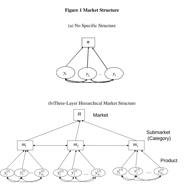
The products are more or less competitive in their market. These products are grouped according to the degree of competitiveness into several segments, and further categorizing these groups to higher levels to make subgroups leads to a hierarchical structure for the market definition. A tree structure is used to represent the hierarchical nature of competitive

relationships among products in a graphical form, as shown in Figure 1. Figure 1(a) indicates the market with no specific structure and each product sale is directly accumulated to market sale. On the other hand, Figure 1(b) shows the situation that some groups of product sales are respectively accumulated to sub-markets first and then sub market sales constitute market sale.

Figure 1 (a), (b) Market Structures

Basic Structure

Let us assume that there are

I

products in the market and that y_it is the number of sales for the product

i

at time

t t

(



1,..., )

T

, which follows the Gamma compound Poisson distribution independently with a time-varying parameter



a

_it

,



_t



defined by (7) for

1,...,

i



I

when there is no competitive relationship with each other. Then, we obtain the Gamma compound Poisson distribution with





a_it,



_t



for market sales, defined as the aggregate of product sales,

1 I t it i n y 





, under the assumption of no specific structure among products in the market, as shown in Figure 1(a). That is, we have marginal distributions for

product and market sales by





~ Compound Poisson , it it t y a



, n_t  Compound Poisson



a_t*,



_t



, (11) where * 1 I t it i

a

a







. Furthermore, after n_t is given, the conditional distribution of product sales

y



_t





y i

_it

,



1,...,

I



follows





| t~ Dirichlet Compound Multinomial t

|

t, t

t n n a

y

y



 , (12)

where

a



_t





a

_1t

,...,

a

_It



'

. The sequential use of equations (11) and (12) produces a joint distribution for market and product sales,







*







, | , | , | ,

t t t t t t t t t t

p n y a



 p n a



p y n a . (13)

We note that the conditioning set



a_t*,



_t,a_t



has equivalent information with



a



_t

,



_t



if we take a_t as a full-dimensional vector with a nondegenerated distribution.

In contrast, Terui et al. (2010) proposed a dynamic generalized linear model based on Poisson variables without over-dispersions. This represents a macromodel for aggregate sales directly without considering the microstructure. They used the reproductive property of Poisson variables and conditional multinomial distribution when the sum of variables is given, and proposed a multivariate time-series model with a hierarchical structure based on the discrete outcomes. That is, we have marginal distributionsy_it Poisson

 



_it and

 

* Poisson

t t

n 



and conditional distribution

y



t

|

n

t



Multinomial



y



t

| ,

n

t t



, where

* 1 I t it i











and _t



_{jt jt} I _it, 1,..., 1



i j I



*

 

*

 



, | , | | ,

t t t t t t t t t

p n y

 

  p n



p y n



 , (14) where the induced parameters *

t

 and  , respectively, represent the expected total sales _t and market shares for each product.

Higher Order Structure

This model is extended to a higher order hierarchical structure, as developed by Terui et al. (2010). Next, we fully explain the model specifications, including the design matrix of state space priors, as this model is applied to actual time-series data in the empirical analysis.

Extending the Poisson–multinomial relationship in the above-described manner, we decompose the market structure into

L

submarkets M_k such that [ ]

1 L _k t _k t

y







_

y



, where





' [ ]

,

k t it k

y





y i



M

represents N_kdimensionalvector of the products that are grouped in

k

M ,

k



1,...,

L

. Given aggregated submarket sales [ ]

,

k k t it i M

m

y







the conditional distribution [ ] [ ] | k k t t

y m ,

k



1,...,

L

, follows independent N_k-dimensionalmultinomial distribution since [ ]k

t

y s are orthogonal to each other, i.e.,



y_t[ ]l |m_t[ ]l

 

 y_t[ ]k |m_t[ ]k



for lk by the definition of a submarket.

Next, let



[1]_,..., [ ]L



_'

t t t

m  m m denote an L-dimensional vector of submarket sales. Then, |

t t

m n follows a multinomial distribution conditional on the sum of submarket sales, i.e., market sales [ ] 1 L k t t k n m 





. In brief, we have a three-layer hierarchical market structure model. We note that

 

y

_t and

 

n

_t are independent, conditional on

 

m



_t . Then, the joint density function of I product sales (bottom layer), L submarket sales (middle layer), and market sales (top layer) are decomposed into





  







 



[ ]

 

[ ] [ ]



1

,

,

|

|

|

|

.

t t t t t t t t L k k k t t t t t k

p n m y

p n p m n p y

m

p n

p m

n p y

m













_

_

 









　　　　　

(15)

Then, we obtain marginal and conditional data distributions: n_t  Poisson

 



_t* ,





| Multinomial , t t t t m n



n



 , where [ ] [ ] 1 1 1

/

j k N L N j k jt it it i k i







  







_

j1,...,L ,1

_





[ ]k _| [ ]k _Multinomial [ ]k _, [ ]k t t t t y m



m





k1,...,L



,



t[ ]k





it[ ]k

,

i

M

k



,







[ ] [ ] [ ] 1

/

k N k k k it it jt j













_

i1,...,N_k1

_

, and



it[ ]k is the parameter of the Poisson variable i

classified to the submarket M_k. The structure of this model is illustrated in Figure 1(b).

5. Data Augmentation Approach to Over-dispersion Data Augmentation

Extending the model for accommodating over-dispersion, instead of direct use of densities (6) and (10), we take a data augmentation approach to keep the original parameters, i.e., implying expected sales and market shares for each product in the modeling, and use the generated sample of augmented variable



*_, '



_'

t t t

z 

 

 in the MCMC process to define the likelihood for the parameters



a_t,



_t



:







*







| , =Gamma | , Dirichlet |

t t t t t t t t

p z a





a







 a . (16)

By using the relation of posterior density











 





 



* * * * * *

,

|

,

, ,

,

|

,

|

|

,

|

,

|

t t t t t t t t t t t t t t t t t t t t t t t t

p a

n y

p a

n y d

d

p n

p

a

d

p y n

p

a d



  

 





 











 



 

 































　　　　　　　

, (17)

we evaluate these integrals by augmenting the gamma and Dirichlet parameters in terms of generating the s-th samples



_t*( )s from gamma



*( )s _| *( )s _, ( )s



t t t

p



a



and



_t( )s from Dirichlet



( )s _{| ,} ( )s



t t t

p



 n a in MCMC iterations. Then, conditional on ( )s



*( )s _, ( )s _{' '}



t t t

z 





 , we



*( )



| s

t t

p n



p y n



_t| _t,



_t( )s



, (18) and this forms a building block to constitute a hierarchical structure.

In case of two-layer models and three submarket (L=3), it is extended as follows: for



* ' [1] [2] [3]



,

,

',

',

' '

t t t t t t

z



  













,











 





 





 



* * * * [ ] [ ] [ ] [ ] [ ] [ ] 1

,

|

,

,

, ;

|

,

,

|

|

,

|

,

|

|

,

|

,

t t t t t t t t t t t t t t t t t t L k k k k k k t t t t mt t t t t t t t k

p a

n m y

p a

z n m y

dz

p n

p

a

d

p m

n

p

a

d

p y

m

p

a

d









 























_

_























 



 





















(19) where

,

1,...,

k mt it i M

a

a k

L











_



_









and a_t[ ]k 



a i_it, M _k



.

We evaluate these integrals by augmenting the gamma and Dirichlet parameters z_t in terms of generated samples



_t*( )s from Gamma p





_t*( )s |a_t*( )s ,



_t( )s



,



_t( )s and





_t[ ]( )k s from Dirichlet p





t( )s |n at, mt( )s



and





( ) ( )

[ ]k s

_|

[ ]k s

t t

p





a



, respectively. Then, conditional on



( ) ( ) ( ) ( ) ( )



( )s *s

_,

's

_,

[1]s

_',

[2]s

_',

[3]s

_{' '}

t t t t t t

z





















, we obtain the Poisson–Multinomial likelihood function:



*( )

 

( )





[ ]( ) [ ]( ) [ ]( )



1 | | , | , L s s k s k s k s t t t t t t t t k p n



p m n



p y m



    



    . (20)

6. Model Specification and Joint Posterior Density Dynamic Generalized Linear Model

Using the expectation of product sales leads to

 

it it t

E y



a



. (21) Thus, we interpret that the expected sale is decomposed into an individual mean a_itand a common mean



_t across products. In turn, we model the mean function as

a

_{it t}





f x



_it

,



_it



connecting with marketing mix variables x_it and stochastic error



_it. We specify the structure in more detail as

loga_it  a_ilog



_t x_it'



_it



_it,　i1,...,I . (22)

That is, the individual mean has a product-specific mean a_i and a common time trend log



_t, and it is assumed to be mostly explained by marketing mix variables. We set *

log

it it i

a  a a and denote * _log

t t

    , and then conditional on a_i, we have the dynamic equation

* *

'

it t it it it

a  x   . (23) This constitutes the structural equation





_t



F

_{t t}







v



_t, where



_t 



a_1t*,...,a_It*



' and



*



1 2 = , ,..., , ' t t t It t





 

 

_, t

F

is the matrix defined by the structure on





_t in equation (24), and v_t is the error vector comprising of



_it. As for the dynamic state vector used in the application, we specify the second-order local common trend for *

t

 and the first-order local trend model for the response parameter



_it, i.e.,

* * 1 1 1 1 2 1 3 ; , 1,... , t t t t t t t it it it w w w i I















                　 (24)

and this specifies the system equation





_t



H

_{t t}





_1



w



_t.

Coupled with the data distribution (15), we define the dynamic generalized linear model with the state space prior:

1

,

~

(0, )

,

~

(0,

)

t t t t t t t t t t

F

v

v

N

V

H

w

w

N

W









_

 

























_

_

. (25)

Joint Posterior Density

Under the usual assumption that the prior density for the covariance matrix of structural and system equations

p V W



,





p V p W

   

, we can express the prior distribution as

 

 

 





 







1

 



   

1

,

, ,

|

|

,

, ,

|

,

,

t t i T t t t i t t i t

p

V W

a

p

X

V

a

p

W

a

p V p W









 

_ 











 



. (26)

Next, we set the prior distribution

p a

 

_i of the individual mean parameter a_i by

















2 2 2 2 0 0 0 0 | , / ; , ; / 2, / 2 i i i i i i i a



N a

 

　　a N a b



IG n s . (27) By arranging the term in (22) as c_it  a_i



_it, wherec_it loga_it log



_tx_it'



_it, for

1,...,

t



T

, we constitute the likelihood for the mean a_i conditional on the error variance

2

i



and derive conditional posterior distribution p a



_i|

 



_t ,

 



_t , ,V W,

 

a_i ,



_i2



in a closed form as 2 2 2 2 2

|

i i i

,

i i i i i

a

Tc

v

a v

N

T

T















_

_











, (28) where 1 / T i it t c c T  



 and

 

a

i means the set of

a k

k

,



1,...,

I

excluding

a

i.

Finally, we obtain the joint posterior density with data augmentation of



* [1] [ 2] [3]



, ', ', ', ' ' t t t t t t z 

  

 







 by equation (29):

 

 



  

   







 

 











 





 



 



   

 

 

 





 

 

2 3 * * [ ] [ ] [ ] 1 1 1 2 2 1 , , , , , ; | data | | , | , | , | , | , | , , , | , | , , , , , . t t i i t k k k T _{t t t t t t t t t t t t t t t t t} k t t t t i t t I i t t i i i i i p V W a z p n p p m n p p y m p p X V a p W p V p W p a V W a p a p









  



  





 





 









          _{ } _    







              　　 (29)

In (29), “data” means the observed data



   

y



_t

,

x



_t



.

of the Poisson–Multinomial distribution perturbed by the Gamma–Dirichlet distributions.

7. Estimation and Forecasting Sampling the link function for MCMC

In addition to the standard Bayesian inference on state space modeling by dynamic linear models (DLMs) by West and Harrison (1997), we use the MCMC approach to estimate the model by using Metropolis–Hastings sampling specifically for the conditional posterior density of link functions based on the data-augmented representation



_t

|

_t

, , , data

_t





_t

,

_t

,

_t

|

_t





_t

|

_t





_t

|

_t

, ,

_t



_t

p





F





V





p n m y

 

z

p z





p





F





V dz

, (30)

where z_t 



  

_t*, _t', _t[1]',



_t[ 2]',



_t[3]' '



. Once the values of  for equation (30) are given, the _t structural equations coupled with the system equations in their state space priors in equation (25) constitute the conventional Gaussian state space models. The multi-move sampler by Carter and Kohn (1994) and Fruhwirth-Schnatter (1994) is used to sample the state vector

 





_t . We assume that the initial values of the state vector



₀ follow a multivariate normal

distributionN





₀,dI



. The mean vector



₀ was set as the estimate of the coefficient on static regression, i.e., the regression with time-invariant coefficient, and we set d = 0.1 for the empirical application.

Predictive Density



 















1 1 1 1 1 1 1 1

|

, data

|

,

|

, ,

, data

|

, ,

, data

,

,

T T T T T T T T T T

p

y

z

p z

p

V W

p

V W

p V W d

dVdW





_









       





_

_

_

_









　　　　

(31)

where

p







_T1

|





_T1

, ,

V W

, data



is the conditional predictive density of link parameters when the predicted state vector, and structural and system error covariance matrices are given. The MCMC method is applied to evaluate this predictive density by the augmenting procedure. To evaluate this density, we first extend equation (16) to define the predictive likelihood of

1 T





 conditional on





T1 by





















* * 1 1 1 1 1 1 1 1 3 [ ] [ ] [ ] 1 , 1 1 1 1 1 1 | , , , , data Gamma | , Dirichlet | Dirichlet | T T T T T T T T k k k T m T T T T T k p z V W a d a a d d





















                







          　　 (32)

The details of the sampling scheme for MCMC are described in the appendix.

8. Empirical Application Data and Variables

We use the store level scanner, point of sales (POS), time series in the curry roux category that was applied to our previous model in Terui et al. (2010) for comparison with the model with over-dispersion. The weekly series comprises three manufacturers that produce three products each, for a total of nine products during 110 weeks.

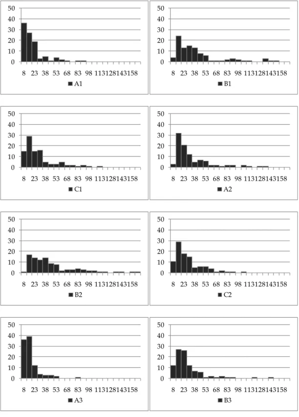
Table 1 Summary of Data

Figure 2 Histogram of Weekly Product Sales Data

Table 1 describes the summary statistics for sales, price display, and feature data. In particular, sales data contains variance to give an evidence of the presence of over-dispersion

in the data. Figure 2 show the histogram of brand sales.

The first 100 weeks are used for estimation and the last 10 weeks are reserved for validation of forecasting. The data contain the amount of product sales for

 

y_it , and “prices”, “display (in-store promotion)”, and “features (advertising in newspaper)” for marketing mix variables

 

x_it . x_it contains not only variables of their own, but also those with other products. The display and features are binary data taking a value of “1” when it was on and “0” when it was off. The logs of price data are used.

Model Comparison

Each of the three makers, A, B, and C, produces three categories of products according to the level of spiciness to accommodate the difference in consumer tastes (1: Not spicy, 2: Medium spicy, 3: Spicy). Following the discussion of Terui (2011), we assume three possible market structures: (1) product category, (2) makers, and (3) usage, i.e., “ordinary” or “luxury” usage, as shown in Figure 3, and compare these models with over-dispersion and without over-dispersion. That is, we have six models to be compared.

Figure 3 Comparative Models

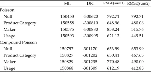
The top of Table 2-1 shows the log of marginal likelihood (LML) as an in-sample fit criterion and two types of predictive measures, i.e., the deviance information criteria (DIC) by Spiegelhalter et al. (2002), and the root mean squared errors (RMSE) of 10-step-ahead forecasts of hold-out samples as out-of-sample criteria.

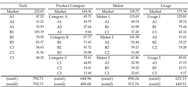
There are three levels for forecasting the RMSE: market, submarket, and product. These errors, including the null model of “no” structure, are reported in the lower panel of the table 2-2. We apply two types of measures: “sum1” and “sum2.” “sum1” is the sum of all errors

induced by the model in which we have no specific preference on the levels to be predicted. “sum2” is defined as the sum of market and product errors by considering that the numbers of submarkets differ between null and other structures.

According to the three criteria, the proposed models based on compound Poisson variables accommodating over-dispersion improve the models with no over-dispersions. In particular, the compound Poisson variable model under the market structure (3) shows the best performance.

Table 2-1 Model Comparison: Overall

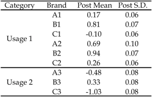
Table 2-2 Model Comparison: Decomposition of RMSE Table 3 Estimates of Product Intercept

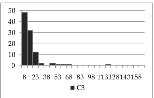
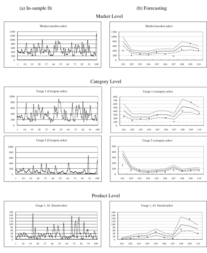
Figure 4 In-sample Performance and Forecasting—Market, Submarket, and Product Figure 5 Estimates of Structural Parameter

The left panels of Figure 4 show the predicted fit of in-sample data for market, submarket of “usage,” and product levels, where each observation is denoted by a dot and the estimates are connected by straight lines. We observe that the model fits the market sales well over the observational period. The right panel of each element depicts its 10-step-ahead forecasting for these sales, where the mean values of the predicted density at each prediction step are connected by a continuous line, and the 2.5% and 97.5% quantiles of the density at each step are connected by dashed lines. The hold-out samples are denoted by dots in the figure. This shows that the market will gradually expand over the next 10 weeks, and these forecasts are consistent with the movement of hold-out samples. We generate the forecasts keeping the last observation x for the prediction steps. _iT

Figure 5(a), (b) show the trajectory of estimated parameters

 



_t and



a_1t,...,a_9t



. It appears that _t s are fluctuating downward for the first period and then turning upward with local trends around a mean level of 0.9998.



a_1t,...,a_9t



move more heterogeneously with large fluctuations, which should be proportional to the observed discrete outcomes.

Figure 5(c) indicates trends for product A2 and B3 sales, which belong to a different category; it shows the opposite trends. Figure 5(d) depicts the time-varying price coefficient estimates in response to price and promotions (“End” display and “Advertising”). We confirm the competitive relationship between submarkets, and more interestingly, we find that products B1 and C2 are not hostile to A1 in the sense of pricing strategy, as they have the same coefficient sign as that of A1.

9. Concluding Remarks

In this study, we proposed a multivariate time series model for over-dispersed discrete data. Therein, we extended the model with the hierarchical structure by Terui et al. (2010) to accommodate the over-dispersion problem inherent in the modeling of market structure based on sales count dynamics. We first discussed the mechanism of the microstructure for generating over-dispersion in a number of discrete sales data.

The Gamma compound Poisson variable for product sales count responses and Dirichlet compound multinomial variables for product share are connected in a hierarchical fashion as a tree structure for depicting a market. The model is based on the likelihood generated by decomposing sales count response variables according to the degree of competitiveness among products and conditioning on their sum, and builds them up to higher levels, represented as a tree structure. State space priors are applied to the likelihood generated by the compound distributions to develop dynamic generalized linear models for discrete responses with a

hierarchical structure.

We first showed that over-dispersion is inherent to the problems where consumers are more or less dependent. Then, we model the compound distributions for accommodating over-dispersions. However, instead of the direct use of the density function of compound distributions, we augment variables to make the numerical integrations for mixing easier, and provide more efficient algorithms compared to the method that makes direct use of compound distributions. The empirical analysis by weekly product sales data in a store showed that our modeling worked well and the models with over-dispersion, which is constructed by compound Poison variables, performs better than the models without over-dispersion.

There are a few problems for future research. One is the extension of the theoretical study. The zero-inflated Poisson (ZIP) model by, for example, Lambert (1992) could be also applied to our modeling when the data contain many zeros. In particular, this could be important if we further incorporate modeling of individual consumer behavior in the analysis. This could be accommodated by mixture distributions through hierarchical models, as used in this study. However, this additional mixture modeling demands more complicated computation procedures. The expected gains from this extension could not be substantial, compared with the development of a new model, and thus, we would like to leave this modification of the model for future research.

Appendix: MCMC Algorithm A.1 Dynamic Generalized Linear Model

We summarize the prior and conditional posterior distribution used for our proposed model below.

Conditional Posterior Distribution

We run 10,000 MCMC iterations in the model. In all models, we used the last 5,000 iterations to estimate the posterior distribution of model parameters. When the initial values of the parameters are given, the conditional posterior density of the necessary parameters is generated as follows.

(i)



_t| t



 is defined by equation (23), and we use Metropolis–Hastings with a random walk algorithm,





( ) ( 1)

0 0 1

s s t t

N

I



_

_



_



_{ }







_

_{ }

, where

I

is an identity matrix with corresponding dimensions.

Acceptance probability



is defined as



( ) ( 1)



_



( ) ( ) ( )



_

( 1) ( 1) ( 1)

|

,

,

, data

,

min

,1

|

,

,

, data

s s s t t t s s t t _{s s s} t t t

p

F

V

p

F

V





  





   































.

After obtaining the draw of these parameters, we use West and Harrison’s (1997) standard Bayesian inference procedure on state space modeling by DLM.

(ii)



t|

The multi-move sampler by Carter and Kohn (1994) and Fruhwirth-Schnatter (1994) is used to sample the state vector

 





_t

(iii)



t*|

Generate



_t*( )s from gamma



*_| *( )s _, ( )s



t t t

p



a



(iv)



t |

Generate



_t( )s from Dirichlet p





t |n at, mt( )s



(v)





_t[ ]k

|



Generate





_t[ ]( )k s from Dirichlet

p







_t[ ]k

|

a



_t[ ]k( )s



Generate

a

_i( )s from 2 2 0 0 2 2 0 0

,

i

,

b a

ma

N

b

m

b

m



   









_

_







where 1 / m i i a_ a m 





. We set a₀ 0,b₀ 10 in the empirical analysis. (vii)



_i2

|



Generate



_i2( )s from _{0 0}





2 1

(

) / 2,

/ 2 .

m i i

IG

n

m

s

a

a

 



_



_

_























We set n₀ 2,s₀ m in the empirical analysis.

A.2 Forecasting Discrete Outcomes and Constituting Predictive Density Given the s-th draw of MCMC







_T( )s

,

V

( )s

,

W

( )s



,

(i) obtain the forecast ( ) 1

s T

 _ from

p







_T₁

|





_T₁

, ,

V W

, data



p







T1

|





T

, ,

V W

, data



by the algorithm of Gaussian state space model; (ii) obtain the forecast ( )

1 s T

z _ from

p z





_T1

|





_T1



to get the parameter





( ) * ( ) ( ) [1] ( ) [ 2] ( ) [3] ( ) 1 1 , 1 ', 1 ', 1 ', 1 ' ' s s s s s s T T T T T T z _ 



_



 _



_



_



_ ;

(iii) generate the random number ( )



* ( )



1 Poisson 1

s s

T T

n _ 



_ for the market sales forecast; (iv) given ( )

1 s T

n _ together with the parameter values



( )



1 s iT



_ , generate ( ) 1 s T m _ by sampling from the multinomial distribution





( ) ( ) ( ) ( ) 1 | 1 Multinomial 1 , 1 s s s s T nT nT T

m  







  for the submarket sales forecasts;

(v) given [ ]( ) 1

k s

t

m  together with the parameter values



1[ ]( )



k s T





 of the multinomial

distribution of submarket M_k, generate the respective product’s forecasts by sampling from the multinomial distribution





[ ]( ) [ ]( ) [ ]( ) [ ]( ) 1 1 1 1

|

Multinomial

,

k s k s k s k s T T T T

y





m







m









 for k=1, …, L;

(vi) iterate steps (i)–(v) M times.

Then, the empirical distribution of



y



_t1[ ]( )k s

,

s



b

,...,

M



approximates the predictive density (31) in [ ]

1 1

k

T t

z _  y_ . We set the burn-in parameter b = 5,000 and the total number of iterations M = 10,000 for the empirical application after checking the convergence. Seven hours of computation were necessary to implement our empirical analysis. By extending the

above forecasting steps up to H step ahead, we obtained the MCMC sample path



[ ]( ) [ ]( ) [ ]( )



1

,

2

,...,

k s k s k s

t t t H

References

Bearden,W.O. and Etzel, M.J. (1982), “Reference group influence on product and brand purchase decisions,” Journal of Consumer Research, vol. 9, pp. 183-194.

Cargnoni, C., Muller, P. and West, M. (1997), “Bayesain forecasting of multinomial time series Through Conditionally Gaussian Dynamic Models,” Journal of the American Statistical Association, vol. 92, pp. 640-647.

Carter, C.K. and Kohn, R. (1994), “On Gibbs sampling for state space models,” Biometrika, vol. 81, pp.541-553.

Fruhwirth-Schnatter, S. (1994), “Data augmentation and dynamic linear models,” Journal of Time Series Analysis, vol. 15, pp. 193-202.

Harvey, A.C. and Fernandes, C. (1989), “Time series models for count or qualitative observations,” Journal of Business and Economic Statistics, vol. 7, pp. 407-422.

Hoadley, B. (1969), “The compound multinomial distribution and bayesian analysis of categorical data from finite populations,” Journal of the American Statistical Association, vol. 64, pp. 216-229.

Hyman, H.H. (1942), “The psychology of status.” Archives of Psychology, 269, 5-91. Reprint in H. Hyman & E. Singer (Eds.), Readings in reference group theory and research (pp. 147-165). New York: Free Press, London: Collier-Macmillan Limited. (Page citations are to the reprint edition).

Lambert, D. (1992), “Zero-inflated Poisson regression, with application to defects in manufacturing,” Technometrics, vol. 34, pp. 1-14.

Ord, K., Fernandes, C., and Harvey, A.C. (1993), “Time series models for multivariate series of count data,” Ed. T. Subba Rao, Developments in Time Series Analysis, pp. 295-309. Park, C.W. and Lessig, V.P. (1977), “Students and housewives: Differences in susceptibility to

reference group influence,” Journal of Consumer Research, vol. 4, pp. 102-110.

Spiegelhalter, D.J., Best, N.G., Carlin, B.P., and van der Linde, A. (2002),“Bayesian measures of model complexity and fit,” Journal of the Royal Statistical Society Series B., vol. 64, pp. 583-639.

Terui, N., Ban, M., and Maki, T. (2010), “Finding market structure by sales count dynamics - multivariate structural time series models with hierarchical structure for count data -,” Annals of the Institute of Statistical Mathematics, vol. 62, pp. 92-107.

Rossi, P, E, G. Allenby and R. McCulloch (2005), Bayesian Statistics in Marketing, John Wiley & Sons, New Jersey.

West, M. and Harrison, P.J. (1997), Bayesian Forecasting and Dynamic Models, 2nd ed., Springer-Verlag, New York.

Bayesian forecasting,” Journal of the American Statistical Association, vol. 80, pp. 73-97. Winkelmann, R. (2008), Econometric Analysis of Count Data (Fifth edition), Springer,

Table 1 Summary of Data

Table 2-1 Model Comparison: Overall

ML: the log of marginal likelihood, DIC: Deviation information measure RMSE: the root mean squared errors of 10 step ahead forecasts

weekly weekly weekly

Brand Price (/100g) Display Feature

Average (Variance) Average Average Average

A1 33.74 (1057.47) 90.04 2.09 0.40 B1 74.11 (4287.59) 90.33 2.10 0.40 C1 51.29 (2034.13) 89.59 2.09 0.40 A2 61.54 (2915.08) 87.29 1.52 0.23 B2 87.00 (4470.92) 83.71 2.73 0.23 C2 49.67 (1551.92) 80.62 3.39 0.20 A3 27.22 (578.82) 101.22 0.69 0.19 B3 48.13 (1947.57) 99.31 0.73 0.19 C3 24.42 (959.64) 99.03 0.72 0.18 weekly Sales

ML DIC RMSE(sum1) RMSE(sum2)

Poisson Null 150453 -300620 792.71 792.71 Product Category 150558 -300810 648.96 480.06 Maker 150575 -300880 858.24 515.76 Usage 150593 -300995 621.13 449.51 Compound Poisson Null 150797 -301170 653.99 653.99 Product Category 150827 -301202 650.41 467.65 Maker 150829 -301235 770.48 490.00 Usage 150868 -301309 612.19 412.85

Table 2-2 Model Comparison: Decomposition of RMSE

Market 222.65 Market 164.36 Market 138.73 Market 171.34

A1 47.52 Category A 65.71 Maker 1 133.65 Usage 1 125.81

A2 31.21 A1 45.75 A1 49.74 A1 38.74 A3 76.93 A2 27.64 B1 62.98 B1 75.44 B1 105.19 A3 9.66 C1 37.20 C1 42.16 B2 78.92 Category B 67.77 Maker 2 141.38 A2 19.21 B3 83.77 B1 71.43 A2 52.44 B2 33.27 C1 54.63 B2 47.72 B2 59.21 C2 19.28 C2 51.56 B3 35.98 C2 31.08

C3 40.32 Category C 35.41 Maker 3 67.46 Usage 2 45.81

C1 44.85 A3 22.50 A3 17.19

C2 19.01 B3 39.22 B3 23.71

C3 13.68 C3 22.65 C3 9.17

(sum1) 792.71 (sum1) 648.96 (sum1) 858.24 (sum1) 621.13

(sum2) 792.71 (sum2) 480.06 (sum2) 515.76 (sum2) 449.51

Poisson

Null Product Category Maker Usage

Market 305.95 Market 215.32 Market 198.35 Market 203.94

A1 42.34 Category A 49.88 Maker 1 124.41 Usage 1 139.20

A2 93.88 A1 20.04 A1 29.99 A1 26.89 A3 55.41 A2 20.69 B1 63.23 B1 30.30 B1 28.20 A3 25.07 C1 35.25 C1 21.26 B2 52.06 Category B 81.87 Maker 2 75.66 A2 16.61 B3 15.59 B1 50.56 A2 17.35 B2 29.37 C1 22.97 B2 32.68 B2 47.74 C2 20.50 C2 27.33 B3 33.89 C2 13.26

C3 10.26 Category C 51.01 Maker 3 80.41 Usage 2 60.14

C1 25.87 A3 14.96 A3 22.01

C2 19.19 B3 47.40 B3 20.79

C3 24.34 C3 22.47 C3 21.18

(sum1) 653.99 (sum1) 650.41 (sum1) 770.48 (sum1) 612.19

(sum2) 653.99 (sum2) 467.65 (sum2) 490.00 (sum2) 412.85

Compound Poisson

Table 3 Estimates of Product Intercept

Category Brand Post Mean Post S.D.

A1 0.17 0.06 B1 0.81 0.07 C1 -0.10 0.06 A2 0.69 0.10 B2 0.94 0.07 C2 0.26 0.06 A3 -0.48 0.08 Usage 2 B3 0.33 0.08 C3 -1.03 0.08 Usage 1

Figure 1 Market Structure (a) No Specific Structure

(b)Three-Layer Hierarchical Market Structure

…

n

1 y 2 y … yI

n

1 y 2 y yI … _… … Market Submarket (Category) Product [1] 1 y 1 [1] N y

n

1

m

m

₂

m

₃ [1] 2 y [2] 1 y y[2]₂ y1[3] [3] 2 y 2 [2] N y 3 [3] N y

Figure 2 Histogram of Weekly Product Sales Data 0 10 20 30 40 50 8 23 38 53 68 83 98 113128143158 A1 0 10 20 30 40 50 8 23 38 53 68 83 98 113128143158 B1 0 10 20 30 40 50 8 23 38 53 68 83 98 113128143158 C1 0 10 20 30 40 50 8 23 38 53 68 83 98 113128143158 A2 0 10 20 30 40 50 8 23 38 53 68 83 98 113128143158 B2 0 10 20 30 40 50 8 23 38 53 68 83 98 113128143158 C2 0 10 20 30 40 50 8 23 38 53 68 83 98 113128143158 A3 0 10 20 30 40 50 8 23 38 53 68 83 98 113128143158 B3

Figure 3 Comparative Models

Three makers produce three categories of products and they are classified into two groups by their usages.

0 10 20 30 40 50 8 23 38 53 68 83 98 113128143158 C3 A B C 1 A1 B1 C1 2 A2 B2 C2 3 A3 B3 C3 2 1 Maker Usage Product Category

Figure 4 In-sample Performance and Forecasting: Market, Submarket, and Product (a) In-sample fit (b) Forecasting

Market Level Category Level Product Level 0 200 400 600 800 1000 1200 1400 1 10 19 28 37 46 55 64 73 82 91 100

Ma rket (ma rket sa les)

0 200 400 600 800 1000 1200 101 102 103 104 105 106 107 108 109 110

Ma rket (ma rket sa les)

0 200 400 600 800 1000 1 10 19 28 37 46 55 64 73 82 91 100

Usa ge 1 (Ca tegory sa les)

0 100 200 300 400 500 600 700 800 101 102 103 104 105 106 107 108 109 110

Usa ge 1 (ca tegory sa les)

0 200 400 600 800 1000 1 10 19 28 37 46 55 64 73 82 91 100

Usa ge 2 (Ca tegory sa les)

0 100 200 300 400 500 101 102 103 104 105 106 107 108 109 110

Usa ge 2 (ca tegory sa les)

0 20 40 60 80 100 120 140 160 180 1 10 19 28 37 46 55 64 73 82 91 100

Usa ge 1, A1 (bra nd sa les)

0 20 40 60 80 100 120 140 160 180 101 102 103 104 105 106 107 108 109 110

Figure 5 Estimates of Structural Parameter (a)

 



_t (b)

 

a

_it 0 50 100 150 200 250 300 1 10 19 28 37 46 55 64 73 82 91 100

Usa ge 2, B3 (bra nd sa les)

0 50 100 150 200 250 300 101 102 103 104 105 106 107 108 109 110

Usa ge 2, B3 (bra nd sa les)

0.9995 0.9996 0.9997 0.9998 0.9999 1.0000 1 10 19 28 37 46 55 64 73 82 91 100 Market, Tau 0.00 50.00 100.00 150.00 200.00 250.00 300.00 1 10 19 28 37 46 55 64 73 82 91 100 Usage1 A1 0.00 50.00 100.00 150.00 200.00 250.00 300.00 1 10 19 28 37 46 55 64 73 82 91 100 Usage1 B1 0.00 50.00 100.00 150.00 200.00 250.00 300.00 1 10 19 28 37 46 55 64 73 82 91 100 Usage1 C1 0.00 50.00 100.00 150.00 200.00 250.00 300.00 1 10 19 28 37 46 55 64 73 82 91 100 Usage1 A2

(c) Trend 0.00 50.00 100.00 150.00 200.00 250.00 300.00 350.00 400.00 1 10 19 28 37 46 55 64 73 82 91 100 Usage1 B2 0.00 50.00 100.00 150.00 200.00 250.00 300.00 1 10 19 28 37 46 55 64 73 82 91 100 Usage1 C2 0.00 50.00 100.00 150.00 200.00 250.00 300.00 1 10 19 28 37 46 55 64 73 82 91 100 Usage2 A3 0.00 50.00 100.00 150.00 200.00 250.00 300.00 1 10 19 28 37 46 55 64 73 82 91 100 Usage2 B3 0.00 50.00 100.00 150.00 200.00 250.00 300.00 1 10 19 28 37 46 55 64 73 82 91 100 Usage2 C3 0.39 0.40 0.40 0.40 0.40 0.40 0.41 0.41 0.41 1 10 19 28 37 46 55 64 73 82 91 100

Usage 1, A2, Trend

0.10 0.10 0.10 0.10 0.10 0.10 0.10 0.10 1 10 19 28 37 46 55 64 73 82 91 100 Usage 2, B3, Trend

(d) Response Parameters -0.03 -0.02 -0.01 0.00 0.01 0.02 0.03 1 10 19 28 37 46 55 64 73 82 91 100

Usage 1, A1, Price coef

A1 B1 C1 A2 B2 C2 -0.03 -0.02 -0.02 -0.01 -0.01 0.00 1 10 19 28 37 46 55 64 73 82 91 100

Usage 2, B3, Price coef

A3 B3 C3 -0.06 -0.04 -0.02 0.00 0.02 0.04 0.06 0.08 0.10 1 10 19 28 37 46 55 64 73 82 91 100

Usage 1, C2, End coef

A1 B1 C1 A2 B2 C2 -0.10 -0.05 0.00 0.05 0.10 0.15 1 10 19 28 37 46 55 64 73 82 91 100 Usage 1, C2, Ad coef A1 B1 C1 A2 B2 C2