Alaska: Insight From Anisotropic Tomography
著者
Tao Gou, Dapeng Zhao, Zhouchuan Huang,
Liangshu Wang
journal or
publication title
Journal of geophysical research: Solid Earth
volume
124
page range
1700-1724
year
2019-02-08
URL
http://hdl.handle.net/10097/00127013
Aseismic Deep Slab and Mantle Flow Beneath Alaska:
Insight From Anisotropic Tomography
Tao Gou1,2 , Dapeng Zhao1 , Zhouchuan Huang2 , and Liangshu Wang2
1Department of Geophysics, Graduate School of Science, Tohoku University, Sendai, Japan,2School of Earth Sciences and
Engineering, Nanjing University, Nanjing, China
Abstract
We present high‐resolution 3‐D images of P wave velocity (Vp), azimuthal anisotropy (AAN), and radial anisotropy (RAN) down to 900‐km depth beneath Alaska obtained by inverting a large number of high‐quality arrival time data from local earthquakes and teleseismic events simultaneously. Our results show that the high‐Vp Pacific slab has subducted down to 450‐ to 500‐km depths. A prominent slab gap is revealed at depths of 65–120 km near the Wrangell volcanic field, which is likely a slab tear acting as a channel that provides ascending mantle materials to generate magmas feeding the surface volcanoes. In the back‐arc mantle wedge near the eastern slab edge, the AAN exhibits trench‐parallel fast‐velocity directions (FVDs), which may reflect along‐strike mantle flow. The FVDs in the subducting Pacific slab are nearly east‐west, which may indicate fossil anisotropy formed at the mid‐ocean ridge. A negative RAN is revealed within the subducting slab, which may be caused by the fast plate subduction with a steep dip angle. Trench‐normal FVDs of the AAN are revealed in the mantle below the Pacific slab, which may reflect mantleflow entrained by the subducting slab. A positive RAN is revealed in the mantle beneath the Yakutat slab, indicating that its shallow subductionflattens the mantle flow below the slab to be subhorizontal. Along‐strike FVDs of the AAN around the eastern slab edge may indicate the edge‐induced toroidal mantleflow.1. Introduction
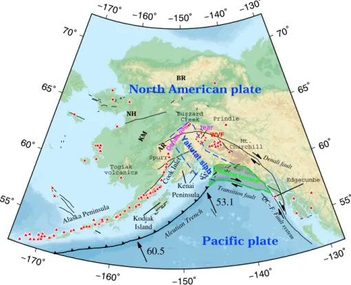
The Alaska mainland region is located in the northeastern Pacific Rim. This region and the Aleutian Islands to the west are the site of northwestward subduction of the Pacific plate beneath the southern margin of the North American plate along the Aleutian megathrust, known as the Aleutian‐Alaska subduction zone. The convergence rate of the Pacific plate with respect to the North American plate is ~50 mm/year at the eastern end of the Aleutian trench and gradually increases along the trench westward (DeMets et al., 1994; Figure 1). As a result, abundant seismicity, active volcanism, and plate boundary deformation occur in this complex subduction system (Plafker & Berg, 1994).
The Alaska subduction zone is tectonically complicated and worthy of study to understand subduction dynamics along a slab edge. Accreted exotic terranes here have been transported by long distances due to convergence and emplaced in their present positions, characterizing the complicated geological environ-ments of Alaska (Moore & Box, 2016; Nokleberg et al., 1994; Plafker & Berg, 1994). The recently accreting Yakutat terrane (Figure 1), bounded by several fault systems as a“corner” geometry, especially the dextral strike‐slip Fairweather fault on the east and the Transition fault on the south, is responsible for the active tectonic process along the northern Gulf of Alaska (e.g., Enkelmann et al., 2009; Haynie & Jadamec, 2017; Jadamec et al., 2013; Koons et al., 2010; Plafker & Berg, 1994). The Yakutat terrane has partially subducted under south central Alaska along with the Pacific slab, at a northwestward rate of ~45.6 mm/year parallel to the Fairweather fault (Fletcher & Freymueller, 2003). Previous studies have suggested that the subducted portion of the Yakutat terrane (i.e., the Yakutat slab) dips at a low angle with a thick low‐velocity (low‐V) and high Vp/Vs seismic feature associated with an oceanic plateau and may be attached to the Pacific slab (Bauer et al., 2014; Eberhart‐Phillips et al., 2006; Ferris et al., 2003; Kim et al., 2014; Qi, Zhao, Chen, & Ruppert, 2007; Rondenay et al., 2008; Rossi et al., 2006; Worthington et al., 2012). The collision between the Yakutat terrane and the North American plate leads to a series of tectonic processes, such as seismic activity (Doser & Veilleux, 2009), mountain building and exhumation (Enkelmann et al., 2009), interplate coupling (Reece et al., 2013; Zweck et al., 2002), and absence of volcanism between the Aleutian volcanic arc and the Buzzard Creek Maars, known as the Denali volcanic gap.
©2019. American Geophysical Union. All Rights Reserved.
RESEARCH ARTICLE
10.1029/2018JB016639
Key Points:
• The Pacific slab has subducted down to 450‐ to 500‐km depths beneath Alaska
• A slab gap exists near the Wrangell volcanicfield
• Anisotropies exist in the mantle wedge and subslab mantle, reflecting mantle flow caused by the slab geometry and subduction
Supporting Information:
• Supporting Information S1 • Data Set S1
Correspondence to:
T. Gou and D. Zhao, [email protected]; [email protected]
Citation:
Gou, T., Zhao, D., Huang, Z., & Wang, L. (2019). Aseismic deep slab and mantleflow beneath Alaska: Insight from anisotropic tomography. Journal of Geophysical Research: Solid Earth, 124, 1700–1724. https://doi.org/ 10.1029/2018JB016639 Received 31 AUG 2018 Accepted 12 JAN 2019
Accepted article online 18 JAN 2019 Published online 8 FEB 2019
So far many researchers have used seismic tomography with local‐earthquake data to investigate the 3‐D velocity structure of the crust and upper mantle beneath south central Alaska (e.g., Eberhart‐Phillips et al., 2006; Kissling & Lahr, 1991; Qi, Zhao, Chen, & Ruppert, 2007; Tian & Zhao, 2012; Worthington et al., 2012; Zhao et al., 1995), greatly improving our understanding of seismotectonics, volcanism, and dynamics of this subduction zone. However, these studies could only image the velocity structure down to ~200‐km depth, including the continental crust, the upper mantle wedge, and the shallow upper portion of the Pacific slab. The deeper portion of the Pacific slab and the mantle below the slab are not well sampled by seismic rays from local earthquakes recorded at seismic stations in Alaska in these studies.
To investigate the mantle structure under Alaska, several studies used teleseismic data recorded by the Alaska Regional Network or the uncompleted USArray Transportable Array, both of which are mainly deployed in south central Alaska and the Alaska Peninsula. Engdahl and Gubbins (1987) inferred that a high‐velocity (high‐V) feature of the Pacific slab extends to a depth of >400 km beneath the central Aleutian Islands, but their result is limited to a 2‐D profile. Qi, Zhao, and Chen (2007) used 15,804 P wave relative traveltime residuals from 889 teleseismic events recorded at 78 stations and showed that the Pacific slab reaches a depth of 300–400 km and becomes deeper westward under south central and western Alaska. Martin‐Short et al. (2016) used P and S wave relative traveltime residuals from 288 tele-seismic events recorded at 158 stations and revealed the high‐V Pacific slab subducting down to >400‐km depth beneath south central Alaska. Burdick et al. (2017) determined a global Vp model of mantle tomo-graphy and suggested that the Pacific slab has subducted down to at least 600‐km depth under Alaska. However, these previous tomographic models have a limited resolution, because the seismic stations they used do not cover the entire Alaska region but are mainly distributed in south central Alaska.
Figure 1. Tectonic setting of the study region. The blue dashed line denotes the extent of the subducted Yakutat slab from Eberhart‐Phillips et al. (2006). The green solid line denotes the boundary of the unsubducted Yakutat terrane from Worthington et al. (2012). The square shown in the red dashed line denotes the slab tear area as inferred by Fuis et al. (2008). The arrows show the motion directions of the Pacific plate with respect to the North American plate (NUVEL‐1A; DeMets et al., 1994), and the numbers beside the arrows denote the rates of plate motions (mm/year). The red triangles denote the active and Quaternary volcanoes. WVF = Wrangell volcanicfield; QC‐F. Fault system = Queen Charlotte‐ Fairweather fault system; BR = Brooks Range; NH = Nulato Hills; KM = Kuskokwim Mountains; AR = Alaska Range.
Seismic anisotropy is a useful and seismologically significant physical parameter that usually provides important constraints on the deformation and dynamic processes in the Earth's interior. Anisotropy has been detected in most subduction zones and is thought to originate from different sources, including the overriding plate, the mantle wedge, the subducting slab, and the mantle below the slab (e.g., Long & Silver, 2009; Savage, 1999). Seismic anisotropy in the upper mantle mainly results from the strain‐induced lattice‐preferred orientation (LPO) of anisotropic minerals, primarily olivine (Long & Silver, 2009). Several fabrics of olivine (A‐, B‐, C‐, D‐ and E‐types) have been found to exhibit different relations between the geo-metry of the anisotropic structure and the dominant slip system (Karato et al., 2008), which vary with water content, stress, and temperature. These olivine fabrics generally exhibit a fast axis parallel to the direction of mantleflow, except for B‐type olivine fabric that exhibits a flow‐normal fast axis direction and is favored by high stresses, low temperatures, and the presence of water (e.g., Karato et al., 2008; Kneller et al., 2005). Shear wave splitting (SWS) measurements estimate the fast direction and strength of azimuthal anisotropy directly beneath a seismic station from orientations of the fast and slow polarized S waves and the differen-tial time between them. Analyzing the splitting of core phases such as SKS can provide information on S wave azimuthal anisotropy in the upper mantle, which can be compared with results of P wave azimuthal anisotropy in the same study region. Complex fast directions of SWS are revealed in the Alaska mainland region (Christensen & Abers, 2010; Hanna & Long, 2012; Perttu et al., 2014). Fast directions in dominant NE‐SW (trench‐parallel) orientations are revealed from the 70‐km depth contour of the Pacific slab to as far as Arctic Alaska, which are parallel (or subparallel) to not only the strike of the Pacific slab but also the absolute plate motion of the North American plate. These trench‐parallel SWS results in areas near the subduction zone are generally considered to mainly reflect anisotropy in the mantle wedge due to along‐strike mantle flow (Christensen & Abers, 2010; Hanna & Long, 2012; Perttu et al., 2014). A possible contribution from plate‐scale asthenospheric flow is also suggested (Hanna & Long, 2012; Perttu et al., 2014). Fast SWS directions in dominant NW‐SE (trench‐normal) orientations are revealed from the south of the 70‐km depth contour of the Pacific slab to the Kenai Peninsula, probably relevant to fossil anisotropy in the subducting slab or anisotropy due to entrainedflow beneath the slab (Christensen & Abers, 2010; Hanna & Long, 2012; Perttu et al., 2014). In addition, overwhelmingly null SWS measurements are revealed by Hanna and Long (2012) in a region around 146°W and south of 65°N. The null splitting can result from either limitation of back azimuths parallel to the fast or slow directions or diverse structural settings, such as isotropic mantle, vertical symmetry axis, or small‐scale variations of mantle flow. However, these interpre-tations are questionable based on the SWS measurements alone because of the poor depth resolution of the SWS method.
Geodynamic modeling is helpful to investigate and understand the relation between mantleflow field and seismic anisotropy in subduction zones (e.g., Faccenda & Capitanio, 2012; Hall et al., 2000; Jadamec & Billen, 2010, 2012; Kneller & van Keken, 2007). The Alaska subduction zone is characterized by complicated subduction configurations such as variable slab dips, curved slabs, oblique subduction, and slab edges, which can have different effects on flow geometry (Kneller & van Keken, 2008). Jadamec and Billen (2010) used 3‐D geodynamic models to test two slab geometries with different shapes of the eastern slab edge and then compared theflow dynamics with the SWS results of Christensen and Abers (2010). In their best fitting model, a significant counterclockwise toroidal component of flow is generated from beneath the slab into the mantle wedge around the eastern slab edge, which is considered important to produce complicated anisotropic structure in the upper mantle.
To clarify the origin of seismic anisotropy and have a better understanding of subduction dynamics of the region, it is necessary to investigate the 3‐D anisotropic structure of the Alaska subduction zone, and P wave anisotropic tomography provides a powerful tool for this purpose (see Zhao et al., 2016 for a recent review). However, previous studies of 3‐D anisotropic tomography (Tian & Zhao, 2012; Y. Wang & Tape, 2014) focused on the anisotropic structure down to 200‐ to 250‐km depth and so obtained little information on anisotropy in the deeper mantle under Alaska.
In this study, we perform high‐resolution P wave velocity (Vp) tomography to investigate 3‐D azimuthal and radial anisotropy structures by conducting a joint inversion of abundant local and teleseismic data recorded by the Alaska Regional Network and the Transportable Array deployed recently in Alaska. Compared with the previous tomographic studies, we have collected a much better data set, and the seismic stations we used
10.1029/2018JB016639
Journal of Geophysical Research: Solid Earth
cover the whole Alaska region densely and uniformly. Our tomographic results show clear images of the aseismic parts of the Pacific slab subducting deeply to the mantle transition zone (MTZ) and intriguing features of seismic anisotropy in the crust and mantle. The present study sheds new light on the deep structure and dynamic processes of the Alaska subduction zone.
2. Data
In this study, both P wave arrival times of local earthquakes and P wave relative traveltime residuals of tele-seismic events are jointly used to conduct tomographic inversions. We compile and use three sets of data from the local shallow and intermediate earthquakes (Figure 2b). Thefirst data set contains 372,012 P wave arrival times of 10,311 earthquakes during January 1977 to June 2007 provided by the Alaska Earthquake Center (AEC). The second data set contains 68,324 P wave arrival times of 1,155 earthquakes during February 1977 to December 2014 released by the International Seismological Center (ISC) bulletins. The third data set contains 94,902 P wave arrival times of 2,894 earthquakes during January 2015 to December 2017 released by the Array Network Facility (ANF). To select a best set of events for our tomographic inver-sion, the shallow offshore events are removed from the data sets because of their poor hypocentral locations. Local earthquakes are relocated iteratively before conducting the tomographic inversion. The local earth-quakes are selected according to the following criteria after the relocation process. (1) Each event has at least 10 arrival times of P and S waves; (2) The change of the origin time is≤0.5 s not only in each iteration but also relative to its initial value determined by the seismic network; (3) Changes of the focal depth and epi-central location are≤20 km not only in each iteration but also relative to the initial hypocentral location; (4) Uncertainties of the epicentral location in latitude and longitude are≤5 km, and the focal depth error is≤7 km.
Our teleseismic data set (Figure 3) contains 325,401 P wave arrivals of 15,619 earthquakes during February 1977 to December 2014 released by the ISC and 337,817 P wave arrivals of 3,995 earthquakes during January 2015 to December 2017 released by the ANF. Each of these events was recorded at over 10 stations in the study region. Their epicentral distances are from 30°to 90°. The teleseismic events with magnitudes≥4.5 are selected from the ISC bulletins, and the events≥ M 4.0 are selected from the ANF database.
Figure 2. (a) Distribution of the seismic stations used in this study. The blue squares denote the stations belonging to the Alaska Regional Network, the open squares denote stations that recorded the data released by the Array Network Facility, the red squares denote the stations belonging to the USArray Transportable Array, and the green squares denote the stations belonging to other networks. (b) Distributions of the local earthquakes used in this study in a map view and east‐ west and north‐south vertical cross sections. The blue dots denote events from the data set released by the Alaska Earthquake Center, the black dots denote events from the data set released by the International Seismological Center, and the red dots denote events from the data set released by the Array Network Facility. Note that the horizontal and depth scales are different.
The AEC and ISC data were recorded at 533 Alaska Regional Network stations, whereas the ANF data were recorded at 190 Transportable Array stations, 53 Alaska Regional Network stations, and 22 other permanent stations (Figure 2a). The accuracy of the arrival times is ~0.1 s.
3. Method
The tomographic method of Zhao et al. (1994, 2012) is applied to invert the P wave arrival times of local earthquakes and relative traveltime residuals of teleseismic events simultaneously. This method can deal with a general velocity model in which complex velocity discontinuities exist and seismic velocity changes in three dimensions. To express the 3‐D Vp structure, a 3‐D grid is set up with a lateral grid interval of ~55 km from the surface to 900‐km depth beneath the study region. We take into account the lateral depth variations of the Moho discontinuity from the CRUST 1.0 model (Laske et al., 2013). The starting 1‐D model for the tomographic inversion is the CRUST 1.0 model for the crust and uppermost mantle and the iasp91 model (Kennett & Engdahl, 1991) for the deeper mantle. An efficient 3‐D ray‐tracing technique (Zhao et al., 1992) is used to compute theoretical traveltimes and ray paths. For a local‐earthquake ray, the possible multiple paths in certain epicentral distances (e.g., direct and head waves) are taken into account, and the ray path with the minimum traveltime is selected by the ray tracing. The LSQR algorithm (Paige & Saunders, 1982) with damping and smoothing regularizations is used to solve the large but sparse system
Figure 3. Distribution of the teleseismic events used in this study. The blue dots denote the events from the data set released by the International Seismological Center. The red dots denote the events from the data set released by the Array Network Facility. The green lines denote major plate boundaries from Bird (2003).
10.1029/2018JB016639
Journal of Geophysical Research: Solid Earth
of observation equations that relate the traveltime data to the unknown 3‐D velocity and local‐earthquake hypocentral parameters (e.g., Zhao et al., 1994, 2012). Optimal values of the damping and smoothing para-meters are selected based on the trade‐off curves between the root‐mean‐square (RMS) traveltime residuals and the norm of the 3‐D Vp model after conducting many inversions (supporting information Figure S1). In addition, we apply the anisotropic tomography method (J. Wang & Zhao, 2008, 2013) to invert our travel-time data for the 3‐D Vp azimuthal anisotropy (AAN) and radial anisotropy (RAN) structures under the study region. A horizontal axis of hexagonal symmetry in the modeling space is assumed for the AAN, whereas a vertical axis of hexagonal symmetry is assumed for the RAN (J. Wang & Zhao, 2013; Zhao et al., 2016). Because inverting for the 3‐D AAN and RAN requires much better ray coverage than for the 3‐D isotropic structure, a coarser 3‐D grid for Vp anisotropy is set up with a horizontal grid interval of ~78 km and a vertical grid interval of 100 km below 200‐km depth. For the AAN inversion, there are two anisotropic parameters at each grid node, whereas for the RAN inversion, there is one anisotropic parameter at each node (for details, see J. Wang & Zhao, 2013). The isotropic Vp and anisotropic parameters are determined simultaneously by one tomographic inversion. The same damping regularization is applied to the isotropic and anisotropic Vp parameters, but different smoothing regularizations are applied to the isotropic and ani-sotropic parameters. The smoothing regularization for the iani-sotropic part is selected by referring to that of the isotropic Vp inversion, whereas the optimal values of the smoothing parameters are selected based on the trade‐off curves (Figure S1).
4. Analysis and Results
4.1. Checkerboard Resolution Tests
Extensive checkerboard resolution tests (CRTs; Zhao et al., 1992) are conducted to examine the resolution scale of the isotropic tomography with our data set. Wefirst assigned positive and negative Vp anomalies of 4% to the 3‐D grid nodes to construct a checkerboard model and then calculated synthetic local‐earthquake arrival times and teleseismic relative traveltime residuals for the model. To simulate the picking errors, Gaussian noise with a standard deviation of 0.1 s is added to the synthetic data. Figure S2 shows the results of three CRTs with lateral grid intervals of 0.33°, 0.5°, and 0.7° as well as the distribution of hit counts (i.e., number of rays passing through each grid node) at three selected depths of 25, 200, and 500 km. Both the pattern and amplitudes of Vp anomalies are well recovered at most of the grid nodes with large hit counts. In the crust and uppermost mantle (e.g., at 25‐km depth), our tomographic model has a lateral resolution of ~30 km, because of the good coverage of crisscrossing rays from abundant local earthquakes and tele-seismic events. The lateral resolution is 30–50 km in the upper mantle to ~200‐km depth beneath interior and southern Alaska. The checkerboard pattern is also well recovered in broad areas at depths of 200–500 km, except for some edge parts of the study volume where the coverage of teleseismic rays is quite poor.
We also conducted CRTs for the AAN and RAN tomography with lateral grid intervals of 0.5°, 0.7°, and 1.0°. For the AAN tomography, positive and negative anomalies of two azimuthal anisotropic parameters are assigned alternately at the grid nodes in the input model, representing AAN of 4% with orthogonal fast‐ velocity directions (FVDs) of 22.5° and 112.5° at every two adjacent grid nodes. In the input model of CRTs for the RAN tomography, positive RAN (horizontal Vp > vertical Vp, i.e., Vph > Vpv) and negative RAN (Vph < Vpv) anomalies of 4% are assigned alternately to the adjacent grid nodes. Figures S3 and S4 show the recovered images of the checkerboard model for the AAN and RAN tomography, respectively. Compared with the isotropic Vp tomography, determining the 3‐D AAN or RAN requires much better azimuthal or incident coverage of ray paths. Our CRT results for the AAN and RAN tomography show that both the pattern and amplitudes of anisotropic anomalies are well recovered under south central Alaska, and the lateral resolution is ~50 km in the crust and 50–80 km in the mantle.
4.2. P Wave Tomography
The RMS traveltime residual is reduced from 0.636 to 0.526 s after the isotropic Vp tomographic inversion. The variance reduction is 29.6%. The RMS traveltime residual is further reduced to 0.511 s after the RAN inversion and to 0.507 s after the AAN inversion. Following the approach of Zhao et al. (1995), we performed Ftest (Draper & Smith, 1966) to investigate whether the reductions of the RMS residual from the isotropic Vpinversion to the anisotropic inversions are statistically significant or not. The F ratio for the isotropic and
AAN models is 2.79, and the ratio for the isotropic and RAN models is 4.83. The two values are greater than the corresponding critical values (1.02 and 1.03) given by the F probability distribution at the 1% level for the decreases of the degree of freedom. Therefore, we are quite sure that the reductions of the RMS traveltime residual are statistically significant.
Figures 4 and 5 show map views of the obtained isotropic Vp tomography. The Vp images in the crust show strong lateral heterogeneities, which mainly reflect the rough surface topography and other surface geologi-cal features due to the long‐term tectonic processes associated with the plate subduction. There are several crustal low‐Vp anomalies correlating with thick Cenozoic sedimentary basins (Eberhart‐Phillips et al., 2006; Tian & Zhao, 2012; Zhao et al., 1995), such as the Cook Inlet basin, Gulf of Alaska basin, Copper River basin, Middle Tanana basin, and Yukon Flats basin (Figure 4a; Kirschner, 1994). A large low‐Vp zone is revealed in the crust beneath the Wrangell volcanicfield, most likely representing magma chambers under the surface volcanoes. In contrast, major high‐Vp anomalies in the crust well correlate with the mountain ranges that are generally composed of plutons and granites (Tian & Zhao, 2012; Wilson & Labay, 2016). A prominent high‐Vp anomaly belt exists in southwestern Alaska at longitude 155°W, probably related to widespread late Cretaceous‐early Tertiary plutonic and volcanic rocks of the Kuskokwim Mountains and the western Alaska Range (Wallace & Engebretson, 1984). In addition, significant high‐Vp anomalies are imaged under south central Alaska where intense mountain building is taking place due to the shallow subduction of the Yakutat slab (Figures 4a, 6d, and 6e; Eberhart‐Phillips et al., 2006; Ferris et al., 2003; Haynie & Jadamec, 2017; Jadamec et al., 2013; Koons et al., 2010; Mazzotti & Hyndman, 2002). In addition, a high‐Vp anomaly
Figure 4. Map views of isotropic Vp tomography. The layer depth is shown in each map. The red and blue colors denote low and high velocities, respectively. The velocity perturbation (%) scale is shown at the bottom. The black triangles denote the active and Quaternary volcanoes. The red dashed line in (a)–(g) denotes the extent of the Yakutat terrane from Eberhart‐Phillips et al. (2006). The dashed ovals denote the major features revealed by this study. Major Cenozoic sedi-mentary basins are labeled in (a): YF = Yukonflats basin; MT = Middle Tanana basin; CR = Copper River basin; CI = Cook Inlet basin; GA = Gulf of Alaska basin. (a) 10 km; (b) 25 km; (c) 40 km; (d) 65 km; (e) 90 km; (f) 120 km; (g) 160 km; (h) 200 km; and (i) 250 km.
10.1029/2018JB016639
Journal of Geophysical Research: Solid Earth
is revealed beneath the western Brooks Range and Nulato Hills west of 150°W (Figures 4d–4i), perhaps rele-vant to a thick lithosphere there (O'Driscoll & Miller, 2015).
A prominent, continuous high‐Vp zone is visible in the upper mantle under the Alaska Peninsula and cen-tral Alaska (Figures 4–6). This high‐Vp zone is associated with the subducting Pacific slab, and its shallow portion (<200‐km depth) is clearly delineated by the seismicity (Figures 4 and 6), which was also found by the previous tomographic studies (Eberhart‐Phillips et al., 2006; Qi, Zhao, Chen, & Ruppert, 2007; Tian & Zhao, 2012; Zhao et al., 1995). The dip angle of the slab changes along the strike of the trench. The sub-ducting Pacific slab dips at an angle of ~30–40° to ~200‐km depth and then gradually steepens at greater depths beneath the Aleutian volcanic arc (Figures 6a–6c). In the shallow subduction zone beneath the Denali volcanic gap (Figures 6d and 6e), however, the slab is subducting at a slope of 10–20° down to ~100‐ to 150‐km depth and then steepens at an angle of >60°, consistent with the slab geometry indicated by the Wadati‐Benioff deep seismic zone (e.g., Ratchkovski & Hansen, 2002). Slab rollback seems to occur below 250‐ to 300‐km depth especially near the eastern slab edge (Figures 6e and 6h). To the northeast of the Buzzard Creek Maars, the seismicity within the slab almost disappears but the high‐Vp zone extends further northeastward (Figures 4d–4h), which was also revealed by the tomographic results of Y. Wang and Tape (2014) and Martin‐Short et al. (2016). In addition, a high‐Vp zone down to ~100‐ to 120‐km depth exists at the southeast of the Wrangell volcanicfield (Figures 4d–4f, 6g, and 6h), which may reflect the subducting high‐Vp slab below the Wrangell volcanic field (i.e., the so‐called Wrangell slab; Bauer et al., 2014; Y. Wang & Tape, 2014). The Wadati‐Benioff zone steepens and extends to 85‐ to 100‐km depth in this region with much less seismicity than that beneath the Aleutian volcanic arc (Fuis et al., 2008; Stephens et al., 1984), which may reflect either the subducting Pacific slab (Fuis et al., 2008) or the less buoyant extension of the Yakutat slab inferred from recent tremor data (Wech, 2016). However, in the vertical
Figure 5. The same as Figure 4 but for the images at 300‐ to 700‐km depths. The red lines in (i) denote locations of the vertical cross sections shown in Figures 6, 9, and 12. The blue dashed line in (i) denotes the extent of the Yakutat ter-rane from Eberhart‐Phillips et al. (2006). (a) 300 km; (b) 350 km; (c) 400 km; (d) 450 km; (e) 500 km; (f) 550 km; (g) 600 km; (h) 650 km; and (i) 700 km.
cross section F (Figure 6f), the Wadati‐Benioff zone is visible but a high‐Vp anomaly corresponding to the slab is absent. A synthetic resolution test (Figures S13c and S13d) shows that the ray coverage is sufficient to recover the input model. Thus, the Vp of the subducting slab beneath the Wrangell volcanicfield may be not apparently higher than that of the surrounding mantle. Partial melting of the Wrangell slab as suggested by the previous studies (e.g., Finzel et al., 2011; Preece & Hart, 2004) may reduce Vp of the slab beneath the Wrangell volcanic field. In this study, we consider the Wrangell slab to be part of the subducting Pacific slab. Between the two high‐Vp anomalies of the aseismic slab edge and the Wrangell
Figure 6. Vertical cross sections (a–h) of isotropic Vp tomography along the profiles shown in Figure 5i. The red and blue colors denote low‐ and high‐velocity perturbations, respectively, whose scale is shown beside (c). The red dots denote seismicity that occurred within a 20‐km width of each profile (60‐km width for (f)–(h)). The red dashed lines in each cross section represent the 410‐ and 660‐km discontinuities. The red triangles denote the active and Quaternary volcanoes. The dashed ovals denote the major features revealed by this study. The arrows in (h) denote the possible migration directions of mantle material. WVF = Wrangell volcanicfield.
10.1029/2018JB016639
Journal of Geophysical Research: Solid Earth
slab (Figures 4d–4f and 6h), there is an unusual gap below the Wrangell volcanic field at ~65‐ to 120‐km depths, which is discussed in detail in the next section.
Our results show that the aseismic portions (at >200‐km depth) of the Pacific slab have subducted down to a depth of ~500–550 km from ~170°W to ~150°W (Figures 5 and 6). However, because teleseismic rays always travel in a subvertical direction, vertical smearing inevitably occurs in teleseismic tomography. In this study, we have conducted many synthetic tests to make sure whether the deep high‐Vp anomaly is a reliable and robust feature or not (Figure S12). In these tests, a synthetic high‐Vp Pacific slab is set down to different depths from 400 to 500 km. The recovered results show that the subducting high‐Vp slab can be well resolved by our data set and the tomographic inversion. Vertical smearing occurs, but it is not significant and its range does not exceed 100 km in depth when the bottom depth of the synthetic slab changes from 400 to 500 km. Our study confirms that the Pacific slab has subducted down to a depth of 450–500 km below the Alaska Peninsula and central Alaska, and this result is much more robust than any of the previous studies. Our tomography reveals significant low‐Vp anomalies in the crust and mantle wedge beneath the Aleutian volcanic front (Figures 4 and 6a–4c). The low‐Vp zones in the mantle wedge under the back‐arc region extend to a depth of 200–250 km. For offshore areas to the southwest, the low‐Vp anomalies could not be imaged because of the poor resolution there. This feature is coherent with the previous tomographic results in this region (Eberhart‐Phillips et al., 2006; Qi, Zhao, Chen, & Ruppert, 2007; Tian & Zhao, 2012; Zhao et al., 1995) and in other subduction zones (e.g., Conder & Wiens, 2006; Huang et al., 2013; Jiang et al., 2009; Schurr et al., 2006; Zhao et al., 1994, 2012), which indicates the source zone of arc magmatism and volcanism caused byfluids from the slab dehydration and corner flow in the mantle wedge (van Keken, 2003; Zhao et al., 1992). In contrast, there are few low‐Vp anomalies in the back‐arc mantle wedge beneath the Denali volcanic gap where arc volcanism is absent (Figures 4, 6d, and 6e). The cessation of volcanism in this area is suggested to result from the shallow subduction of the Yakutat slab that probably inhibits the magma production and its rise to the surface (Finzel et al., 2011; Rondenay et al., 2010) and perhaps also related to dominantly rapid horizontal toroidalflow beneath the Denali volcanic gap inferred from geodynamic mod-els (Jadamec & Billen, 2010, 2012). As shown in Figure 6, although it is hard to distinguish the Yakutat slab from the surrounding mantle just according to their velocities due to the limited resolution, the seismicity that solely occurs within the Yakutat slab (e.g., Ferris et al., 2003) and the underlying high‐Vp Pacific slab can roughly delineate the slab morphology.
Obvious low‐Vp anomalies are imaged in the mantle wedge and perhaps in the Yakutat slab under the fore‐ arc region. Low‐Vp anomalies exist and extend below the 410‐km discontinuity under southeastern Alaska east of 140°W (Figures 4, 5, and 6h). The Northern Cordilleran slab window may exist beneath this area (e.g., Madsen et al., 2006; Thorkelson & Taylor, 1989), and the low‐Vp feature probably reflects an upwelling plume through this slab window. Previous teleseismic tomography studies (e.g., Frederiksen et al., 1998; Mercier et al., 2009; Qi, Zhao, & Chen, 2007) could not determine the bottom depth of the low‐V feature. Frederiksen et al. (1998) imaged a similar low‐Vp anomaly down to 600‐km depth but with strong vertical smearing. Qi, Zhao, and Chen (2007) revealed a low‐Vp anomaly reaching ~400‐km depth, but their tion test shows a lower resolution there. Considering the degree of vertical smearing revealed by our resolu-tion test (Figure S14), we think that the maximum depth of the low‐Vp upwelling plume is most likely down to the upper MTZ beneath the Mount Edgecumbe volcanicfield. A depression of the 410‐km discontinuity also indicates that the hot upwelling plume originates from the upper MTZ (Dahm et al., 2017). In addition, this low‐Vp anomaly seems to connect with the low‐Vp anomalies beneath the Wrangell slab and within the slab gap (Figure 6h), but its effect on mantle dynamics is unclear.
To confirm the robustness of our results, we also conducted isotropic Vp tomographic inversions using only the AEC and ISC data (Figures S5 and S6) and using only the ANF data (Figures S7 and S8). The tomo-graphic results obtained with the separate data sets reveal the same or very similar features, further indicat-ing that these structural features are reliable and robust.
4.3. P Wave Anisotropy
Map views of Vp AAN and RAN tomography are shown in Figures 7 and 8 and Figures 10 and 11, respec-tively. Varied and complex anisotropies exist in the crust for both the AAN and RAN tomography, which may reflect fossil anisotropy in the overriding plate. In the AAN tomographic results (Figures 7–9), the
FVDs are predominantly NE‐SW (trench‐parallel) in the back‐arc mantle wedge near the eastern slab edge. The AAN in the high‐V subducting Pacific slab dominantly exhibits FVDs aligning in nearly the E‐W or NWW‐SEE direction. It is important to note that the AAN has FVDs in the NW‐SE direction within the Yakutat slab at 65‐ to 90‐km depths, perhaps reflecting anisotropy related to the strike‐slip faults (Figure 1). Below the Pacific slab, the FVDs of the AAN are aligned in the directions from N‐S to NNW‐SSE at depths of 120–300 km. In the RAN tomography, a prominent feature is the overwhelming preponderance of negative RAN (Vph < Vpv) within the high‐V subducting Pacific slab. In addition, the RAN shows a significant transition from positive (Vph > Vpv) to negative beneath the slab within and outside of the Denali volcanic gap. These AAN and RAN features indicate complex anisotropic structures and dynamics of the Alaska subduction zone.
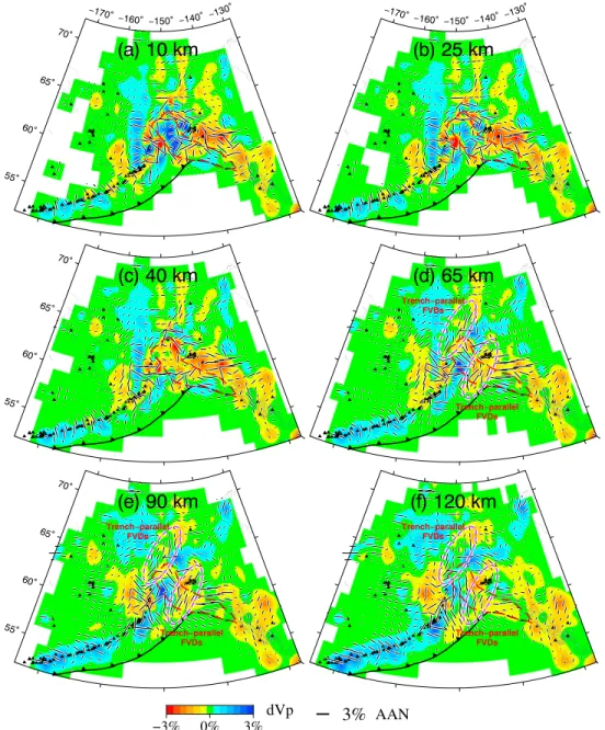
Figure 7. Map views of Vp azimuthal anisotropy (AAN) tomography. The orientation and length of the black bars repre-sent the fast‐velocity direction and the amplitude of AAN, respectively. The dashed ovals denote the major features revealed by this study. The scales of the isotropic velocity perturbation (%) and AAN (%) are shown at the bottom. The other labeling is the same as that in Figure 4. (a) 10 km; (b) 25 km; (c) 40 km; (d) 65 km; (e) 90 km; and (f) 120 km. FVDs = fast‐velocity directions.
10.1029/2018JB016639
Journal of Geophysical Research: Solid Earth
We conducted two synthetic resolution tests to evaluate the reliability of the AAN and RAN tomographic results. The amplitude of anisotropy obtained by the real inversions is normalized to 2% in the input models. As shown in Figures S15 and S16, the FVDs of the AAN are well recovered for most parts of the study volume. In the parts of the model beneath south central Alaska, the AAN amplitudes are also well recovered. Similarly, the RAN pattern and amplitudes are generally well recovered except for western Alaska and some edge portions of the study region (Figures S17 and S18). Some unexpected features of anisotropy appear in the two recovered results, but they have small amplitudes and so are insignificant. The main features of the AAN and RAN models are further examined by performing two simplified synthetic tests (Figures S19 and S20), which show that the anisotropic features can be well recovered.
An important issue of the anisotropic tomography is the possible trade‐off between the Vp anisotropy and heterogeneity. Extensive synthetic tests are performed to investigate this issue. First, a synthetic data set is constructed for an isotropic model that is modified from the obtained 3‐D isotropic Vp tomography
Figure 8. The same as Figure 7 but for the images at 160‐ to 600‐km depths. The red double sided arrows denote a toroidal distribution of the fast‐velocity directions of the azimuthal anisotropy around the eastern slab edge. (a) 160 km; (b) 200 km; (c) 300 km; (d) 400 km; (e) 500 km; and (f) 600 km. FVDs = fast‐velocity directions.
(Figures 4–6). Then the synthetic data are inverted by applying the AAN and RAN tomographic methods, respectively. Finally, the recovered results are compared with the input model.
Figures S21 and S22 show the recovered results for the AAN tomography. Since most of the presupposed anisotropy can be well recovered in the synthetic tests, the trade‐off between the AAN and the isotropic Vpvariation could be greatly reduced if their FVDs are quite different from those in the obtained AAN tomography (Figures 7 and 8). However, it would be difficult to clarify whether the features of anisotropy in the obtained AAN model are reliable or not, when the AAN in the synthetic test has similar FVDs to those in the obtained AAN tomography (Figures 7 and 8). The trade‐off is trivial in the crust (Figures S21a–S21c), thanks to the excellent ray coverage there. A nonnegligible trade‐off occurs in the subslab mantle at 65‐ to
Figure 9. Vertical cross sections (a–h) of Vp azimuthal anisotropy (AAN) tomography along the profiles shown in Figure 5i. The orientation and length of the black bars represent the fast‐velocity direction and the amplitude of AAN, respectively. The scales of the isotropic velocity perturbation (%) and AAN (%) are shown beside (c). The other labeling is the same as that in Figure 6. WVF = Wrangell volcanicfield; FVDs = fast‐velocity directions.
10.1029/2018JB016639
Journal of Geophysical Research: Solid Earth
160‐km depths (Figures S21d–S21g), where the FVDs are similar to those in the obtained AAN tomography. In the deeper areas, we think that the feature of trench‐normal FVDs is reliable and robust, because the trade‐off rapidly decreases with depth (Figures S21h, S21i, and S22a). The trade‐off also occurs at some edge portions of the study region, such as the Alaska Peninsula, western Alaska, and southeastern Alaska (e.g., Figures S21d, S21e, and S22b–S22d), which is expected.
The trade‐off between the RAN and the isotropic Vp variation is shown in Figures S23 and S24. A negative RAN (Vph < Vpv) exists in the subslab mantle beneath southern Alaska at 90‐ to 160‐km depths (Figures S23e–S23g). The patterns of positive RAN (Vph > Vpv) beneath southeastern Alaska east of 140° and the RAN beneath western Alaska (Figures S23 and S24) are also similar to these of the RAN tomographic model (Figures 10 and 11). These RAN features are doubtable due to the consistency of the two models. Only when the trade‐off is rather small and the presupposed anisotropy can be well recovered by the synthetic test, the
Figure 10. Map views of Vp radial anisotropy (RAN) tomography. The length of black bars denotes the RAN ampli-tude. The horizontal and vertical bars represent Vph > Vpv and Vph < Vpv, respectively. The scales are shown at the bottom. The other labeling is the same as that in Figure 4. (a) 10 km; (b) 25 km; (c) 40 km; (d) 65 km; (e) 90 km; and (f) 120 km.
features of the RAN tomographic model can be considered to be reliable, such as the negative RAN within the high‐V Pacific slab (Figure 12).
5. Discussion
5.1. Deep Subduction of the Pacific Slab
The most significant feature in our results is the northwestward dipping high‐Vp zone corresponding to the subducting Pacific slab below the Alaska Peninsula and central Alaska (Figures 4–6). The joint inversion of local and teleseismic data is able to reveal the morphology of the Pacific slab. This result indicates that the aseismic deep portion of the slab has subducted down to a depth of ~450–500 km (Figure 13) even consider-ing the effect of smearconsider-ing as revealed by the synthetic tests (Figure S12). Global tomography (e.g., Zhao et al., 2013) shows that the Pacific slab has reached the MTZ beneath Alaska. Our results indicate that the slab has neither sunk into the lower mantle nor becomes stagnant in the MTZ. The study of Dahm et al. (2017) about
Figure 11. The same as Figure 10 but for the images at 160‐ to 600‐km depths. (a) 160 km; (b) 200 km; (c) 300 km; (d) 400 km; (e) 500 km; and (f) 600 km.
10.1029/2018JB016639
Journal of Geophysical Research: Solid Earth
the topography of the MTZ discontinuities also suggested that the cold Pacific slab has extended from the upper mantle to the upper MTZ but does not penetrate the 660‐km discontinuity beneath central Alaska. Farther to the west, the Pacific plate began to subduct earlier under the North American plate beneath the Aleutian Islands according to global plate reconstructions (Lithgow‐Bertelloni & Richards, 1998). The global tomographic result of Simmons et al. (2012) shows that the Pacific slab seems to penetrate into the lower mantle and the subducted Kula plate became stagnant in the MTZ there. Our tomography shows no signifi-cant high‐Vp feature corresponding to the subducted Kula plate, suggesting that the Kula plate may have sunk into the lower mantle or exist in the MTZ outside of our study region.
5.2. Slab Gap below the Wrangell Volcanic Field
Our results show a prominent gap of the high‐Vp Pacific slab in the vicinity of the Wrangell volcanic field (Figures 4d–4f and 6h). To the northwest of the gap is the aseismic eastern slab edge, and to the southeast of it is the Wrangell slab (Figure 13). We conducted two synthetic tests to investigate whether this gap is a
Figure 12. Vertical cross sections (a–h) of Vp radial anisotropy (RAN) tomography along the profiles shown in Figure 5i. The length of black bars denotes the RAN amplitude. The horizontal and vertical bars represent Vph > Vpv and Vph < Vpv, respectively. The scales are shown beside (c). The other labeling is the same as that in Figure 6.
reliable feature or not (Figure 14), following the approach of Huang et al. (2013) who found a window in the subducting Philippine Sea slab beneath SW Japan (Zhao et al., 2012). Our test results indicate that, if the high‐Vp slab exists there, it can be certainly detected by our data set and tomographic inversion. This feature of slab gap is also visible when only the AEC and ISC data (Figures S5 and S6) or only the ANF data are used (Figures S7 and S8). In this area, our tomography has a high resolution, as shown by the CRTs (Figure S2). Therefore, we are confident that the slab gap indeed exists there.
If the high‐Vp Pacific slab is absent in the gap area, then the gap may be a tear in the Pacific slab (Figure 1) as suggested by Fuis et al. (2008) or a concave jagged slab edge after its separation from the subducted Resurrection plate remnant (Madsen et al., 2006). In contrast, if the Pacific slab is continuous there, the gap may be a result that the low‐Vp oceanic crust of the Yakutat slab overlies the high‐Vp Pacific slab. However, the inferred northeastern boundary of the Yakutat slab just lies about 50–80 km southwest of the gap (Eberhart‐Phillips et al., 2006). Therefore, the gap is most likely due to the absence of the Pacific slab. Furthermore, there is a high‐Vp anomaly connecting with the eastern slab edge at 65‐ to 200‐km depths to the north of the Prindle volcano (Figures 4d–4h). The high‐Vp anomaly seems to be a torn remnant of the Pacific slab and probably had been originally at the position of the current slab gap, but it is also possible that the high‐Vp anomaly is essentially a convex jagged slab edge and the gap is not a slab tear. In this study, we prefer the interpretation that the gap is a tear of the Pacific slab, but the gap in our image looks slightly dif-ferent from the tear as shown by Fuis et al. (2008).
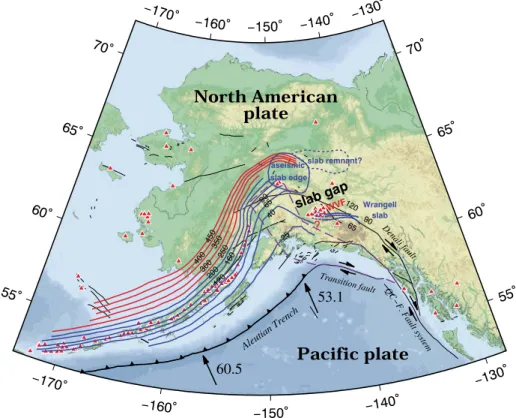
Figure 13. Depth contours to the upper boundary of the subducting Pacific slab and other findings of the present study. The blue lines with depth values denote the slab contours (≤200‐km depth) estimated from both the Wadati‐Benioff zone seismicity and the isotropic Vp tomographic results of this study. The red lines with depth values denote the slab contours (>200‐km depth) estimated from the isotropic Vp tomographic results of this study. Note that the blue dashed lines beneath the Wrangell volcanicfield denote the slab contours inferred from the Wadati‐Benioff zone seismicity there. The blue closed curve denotes the range of the aseismic slab edge. The blue dashed line denotes the range of the slab remnant. The purple dashed line denotes the extent of the Yakutat terrane from Eberhart‐Phillips et al. (2006). The arrows show motion directions of the Pacific plate with respect to the North American plate (DeMets et al., 1994), and the numbers beside the arrows denote the rates of plate motions (mm/year). The red triangles denote the active and Quaternary volcanoes. WVF = Wrangell volcanicfield; QC‐F. Fault system = Queen Charlotte‐Fairweather fault system.
10.1029/2018JB016639
Journal of Geophysical Research: Solid Earth
The slab gap isfilled with a low‐Vp anomaly that is connected with a low‐Vp zone below the Wrangell volcanicfield and extends northeastward until reaching below the Prindle volcano (Figures 4d–4f and 6f). In addition, it is a notable feature that the slab gap is connected with the low‐Vp mantle beneath the slab. The AAN nearby the slab gap exhibits FVDs aligned in the NE‐SW direction at 65‐ to 120‐km depths (Figures 7d–7f), which may indicate mantle flow passing through this gap. SWS observations in the Chile subduction zone (Russo et al., 2010) and some geodynamic models (e.g., Jadamec, 2016; MacDougall et al., 2014; Menant et al., 2016) show that subslab mantleflow near a slab gap can pass through the gap and enter into the mantle wedge. Large variations of the dip and strike of the slab may contribute to drive the subslabflow passing through the gap, as revealed by geodynamic models (MacDougall et al., 2014). In addition, the subslab FVDs aligned in the NE‐SW direction near the gap are parallel to the strike of the deep slab west of ~147°W. This feature is probably consistent with a slab‐edge related upwelling associated with the toroidalflow around the eastern slab edge in south central Alaska (Jadamec, 2016).
The Wrangell volcanism began at about 20–26 Ma and generally becomes younger northwestward (Plafker, 1987; Richter et al., 1990). The presence of adakitic volcanic rocks in the Wrangell area revealed by petrolo-gical analysis of Preece and Hart (2004) indicates slab melting of the young (<20–30 Ma) downgoing slab at shallow depths (75–85 km), exactly consistent with the high‐Vp Wrangell slab. In addition, the subslab mantleflow passing through the slab gap may provide mantle materials and heat to generate adakitic magmas, which is characterized by the low‐Vp anomalies and the NE‐SW FVDs of the AAN below the slab (Figures 7d–7f). We think that the slab gap probably provides a channel to supply magmas for the volcanism in the Wrangell area.
5.3. Slab Contours
There are many slab geometry models of the Alaska subduction zone (e.g., Gudmundsson & Sambridge, 1998; Hayes et al., 2018; Jadamec & Billen, 2010; Syracuse & Abers, 2006; Zhao et al., 1995). These models were mostly obtained by contouring the top surface of the Wadati‐Benioff seismic zone, and so either they have no aseismic portion of the slab or the deep aseismic slab is poorly constrained. In this study, we con-struct a new slab contour model (Figure 13) based on both the Wadati‐Benioff zone seismicity and the high‐Vp subducting slab imaged by our isotropic Vp tomography (Figures 4–6). The aseismic slab edge (Figures 4d–4h) is not contoured because that part of the slab is not very robust. In addition, the subducted portion of the Yakutat terrane (i.e., the Yakutat slab) is regarded as a part of the subducting Pacific slab when contouring the slab beneath the Denali volcanic gap. Our results do not image the Wrangell slab directly beneath the Wrangell volcanicfield where the Wadati‐Benioff zone seismicity exists (Figure 6f) but just in
Figure 14. Two synthetic resolution tests for isotropic Vp tomography. The depth of each layer is shown at the upper left corner of each map. The red and blue colors denote low and high‐velocity perturbations (%), respectively, whose scale is shown at the bottom. The gray triangles denote the active and Quaternary volcanoes. (a) 65 km; (b) 120 km; (c) 65 km; (d) 120 km; (e) 65 km; (f) 120 km; (g) 65 km; and (h) 120 km.
its vicinity. The northern part of the high‐Vp Wrangell slab is located north of the Mount Churchill volcano (Figure 13), which is quite different from the slab geometry suggested by Wech (2016) and the slab model used by Jadamec and Billen (2010) in which the slab only extends to 115‐km depth east of 148°W. 5.4. Anisotropy and Flow Around the Slab Edge
Sinceflow‐normal B‐type olivine fabric is thought to dominantly manifest in the fore‐arc area (Karato et al., 2008; Kneller et al., 2005), we consider that the mantle anisotropy in most parts of the study volume is flow‐parallel. Possible preservation or overwriting of the LPO patterns formed early in the subduction pro-cess due to the time‐dependent rapidly varying flow field may be important to anisotropy in subduction zones (MacDougall et al., 2017), but it is not considered in our discussion because the anisotropic Vp tomo-graphy here is unable to identify anisotropies formed at different stages.
Our results show obvious AAN with dominant FVDs generally parallel to the strike of the subducting Pacific slab in the mantle wedge under the back‐arc areas from 154°W to 145°W (Figures 7d–7f). This feature is well consistent with the observations of the trench‐parallel SWS to the north of the 70‐km depth contour of the Pacific slab at depths of 65–120 km (Figures 15b–15d), which supports the viewpoint that the trench‐parallel anisotropy mainly originates from the mantle wedge (Christensen & Abers, 2010; Hanna & Long, 2012; Perttu et al., 2014; Tian & Zhao, 2012). This feature most likely reflects along‐strike mantle flow, but it is still unclear how the trench‐parallel mantle flow is produced. It was suggested that the flow is either due to the shallow subduction or a toroidalflow around the slab edge (Christensen & Abers, 2010). The latter case is supported by geodynamic models of slab‐driven mantle flow of the Alaska subduction zone, which show counterclockwise toroidalflow around the eastern slab edge and trench‐parallel asthenospheric flow in the mantle wedge north of the 70‐km depth contour of the slab (Jadamec & Billen, 2010, 2012).
Our results suggest that the mantleflow in the eastern slab edge area is induced by the complex slab morphology and seems to exhibit FVDs in a toroidal distribution. The effects of slab dip variations, curved slabs, and slab edges onflow geometry are suggested by geodynamic models (e.g., Kneller & van Keken, 2008). In addition, the steeply subducting slab near the eastern slab edge seems to have some rollback below 250‐ to 300‐km depth in our results (Figures 6e and 6h), which may induce toroidal flow along the slab edge (e.g., Jadamec & Billen, 2012; Schellart, 2004). To the east of the slab edge, the AAN shows FVDs aligned in the NW‐SE direction. A similar feature is revealed by the surface wave tomography of Y. Wang and Tape (2014). Our results also show the FVDs roughly parallel with the slab edge at 65‐ to 500‐km depths (Figures 7 and 8), which may indicate toroidal mantleflow induced by the slab edge extending to a greater depth. Similar toroidalflow around slab edges is also indicated by not only geodynamic models (Schellart & Moresi, 2013) but also SWS observations in a few other subduction zones, such as Kamchatka (Peyton et al., 2001), the Mendocino triple junction (Eakin et al., 2010; Zandt & Humphreys, 2008), and southern Italy (Baccheschi et al., 2011; Civello & Margheriti, 2004), as well as Vp AAN tomography of the Ryukyu‐Taiwan region (Wei et al., 2015, 2016).
5.5. Anisotropy in the Subducting Slab
Our AAN results show that the dominant FVDs are nearly E‐W in the subducting Pacific slab (Figures 7–9). Anisotropy in the subducting slab is usually thought to reflect the fossil fabric formed at the spreading mid‐ ocean ridge (e.g., Zhao et al., 2016). The frozen‐in anisotropy in the oceanic plate is generally consistent with the paleo‐spreading orientations, which is indicated to result from the LPO of aligned anisotropic minerals such as olivine during the formation of the oceanic plate (Collins et al., 2012; Forsyth, 1975; Hess, 1964; Oikawa et al., 2010; Smith et al., 2004). In addition, preferred orientation such as aligned hydrated faults in the slab can contribute to another source of anisotropy (Faccenda et al., 2008). In the Alaska subduction zone, we think that the fault‐induced anisotropy is not likely the dominant mechanism, because the FVDs aligned in nearly the E‐W direction conflict with the trench‐parallel strikes of the faults and cracks in the slab. Considering the orientation of the symmetry axis of anisotropy within the Pacific plate due to the northwestward bending, the original anisotropy would have an NW‐SE (trench‐normal) FVD before the plate subduction, if we assume that the present anisotropy we obtained has not been overprinted by the subduction‐related processes. Recent global AAN models also revealed trench‐normal FVDs in the lithosphere of the Pacific plate before subduction (e.g., Debayle et al., 2016; Schaeffer et al., 2016). The con-sistency of these AAN results in the Pacific plate may indicate that the original frozen‐in anisotropy in the
10.1029/2018JB016639
Journal of Geophysical Research: Solid Earth
slab is well preserved. However, the original FVDs in the Pacific plate are generally oblique to the E‐W paleo‐ spreading orientations in Alaska. The misfit between the FVDs in the oceanic plate and the paleo‐spreading orientations might indicate more complex mechanisms for anisotropy generation at the time of the oceanic lithosphere formation, probably related to the spreading rate, the plate age, or the ancient plate motions (Becker et al., 2014; Takeo et al., 2016).
Our Vp RAN tomography shows that the subducting slab exhibits dominantly a negative RAN (Vph < Vpv; Figures 10–12). This feature is apparently different from the result in Japan that the subducting Pacific and Philippine Sea slabs exhibit a positive RAN (Vph > Vpv; Liu & Zhao, 2017; J. Wang & Zhao, 2013), but it is in good agreement with the Vp RAN model of Hua et al. (2017) that shows a negative RAN in the subducting European and Adriatic slabs beneath the Alps. Hua et al. (2017) suggested that the discrepancy in the dip angle of the subducting slabs beneath the Alps and Japan leads to the RAN difference in the slabs, because the Pacific and Philippine Sea slabs beneath Japan are subducting with a lower angle whereas the European and Adriatic slabs under the Alps have a nearly vertical angle. The deep slab beneath Alaska has also a nearly vertical dip angle and so exhibits a negative RAN (Figure 12), similar to those beneath the Alps. 5.6. Anisotropy and Flow in the Subslab Mantle
The subslab mantle exhibits predominant FVDs of the AAN from N‐S to NNW‐SSE beneath the Kenai Peninsula and its offshore areas at depths of 160–300 km (Figures 7–9). Although a trade‐off occurs between the anisotropy and isotropic Vp at 90‐ to 160‐km depths beneath this region (Figures S21e–S21g), trench‐
Figure 15. Comparison of Vp azimuthal anisotropy (AAN) obtained by this study (blue bars) with average shear wave splitting measurements (red bars) from pre-vious studies (Christensen & Abers, 2010; Hanna & Long, 2012; Perttu et al., 2014). The red crosses denote null measurements of Hanna and Long (2012). The black dashed line in each map denotes the 70‐km depth contour of the Pacific slab. The scales of the AAN amplitude and the shear wave splitting strength (delay time) are shown at the bottom. (a) 40 km; (b) 65 km; (c) 90 km; (d) 120 km; (e) 160 km; (f) 200 km; (g) 300 km; (h) 400 km; and (i) 500 km.
normal FVDs continue to exist at greater depths where the trade‐off is trivial (Figures S21h, S21i, and S22a). Hence, we believe this feature to be reliable and robust. The trench‐normal FVDs in our results have a good match with the fast directions of the SWS measurements to the south of the 70‐km depth contour of the slab (Figures 15d–15h). Possible contributions to the trench‐normal SWS observations are generally suggested to come from the fossil anisotropy in the slab or the anisotropy in the subslab mantle, because the mantle wedge close to the trench is too thin to provide strong enough anisotropy (Christensen & Abers, 2010; Hanna & Long, 2012; Perttu et al., 2014). In addition, Song and Kawakatsu (2013) suggested that the RAN in the subducting asthenosphere formed prior to subduction is a dominant source of seismic anisotropy in central Alaska, and it contributes to the switch of fast polarization direction from trench‐normal to trench‐parallel through the angle of the tilted symmetry axis changing with the slab dip. Our Vp anisotropy results confirm the contribution from the mantle below the downgoing Pacific slab, due to either the subslab mantleflow shown in the geodynamic models of Jadamec and Billen (2010, 2012) or the prior anisotropy within the subducting asthenosphere. In addition, there is also a possibility that the fossil anisotropy within the slab has a secondary contribution to the trench‐normal SWS results, because the FVDs are roughly obli-que or normal to the trench. The trench‐normal FVDs below the slab may reflect the entrained mantle flow due to the downgoing Pacific slab as suggested by the previous studies (Christensen & Abers, 2010; Hanna & Long, 2012; Perttu et al., 2014), but a larger‐scale flow related to the Pacific plate motion is also possible due to the consistency of the FVDs and the absolute plate motion (Perttu et al., 2014). The global AAN models also indicate a goodfit between the FVD in the asthenosphere (at 200‐km depth) and the absolute plate motion of the near‐trench incoming Pacific plate (Becker et al., 2014; Debayle et al., 2016; Schaeffer et al., 2016), which may indicate a large‐scale mantle flow in the NW‐SE direction relevant to the plate motion. It is worth noting that the RAN in the subslab mantle exhibits an abrupt transition from positive (Vph > Vpv) beneath the Denali volcanic gap to negative (Vph < Vpv) beneath the Kenai Peninsula and the offshore areas (Figures 10–12). This feature may indicate a predominantly horizontal mantle flow existing beneath the Yakutat and Pacific slabs, possibly due to the buoyant shallow subduction. In addition, a negative RAN exists in the subslab mantle outside of the Denali volcanic gap. However, although the negative RAN can be well recovered by the synthetic tests (Figures S17 and S18), the resolution test (Figure S23) shows a strong trade‐ off in that area. If the negative RAN beneath the slab is reliable, it may reflect a dominantly vertical mantle flow that is most likely entrained by the subducting Pacific slab.
6. Conclusions
We collected a large number of high‐quality local‐earthquake and teleseismic arrival time data recorded by the Alaska Regional Network and the USarray Transportable Array and determined high‐resolution P wave tomography for 3‐D P wave velocity (Vp), AAN, and RAN down to 900‐km depth under the Alaska mainland region. Our results show clearly that the Pacific slab has subducted down to a depth of 450–500 km below the Alaska Peninsula and central Alaska. An unusual slab gap is detected at 65‐ to 120‐km depths between the aseismic eastern slab edge and the Wrangell slab, which may be a slab tear and provide a channel to supply magmas for the Wrangell volcanoes on the surface. Trench‐parallel FVDs of the AAN are revealed in the back‐arc mantle wedge near the eastern slab edge, probably induced by the along‐strike mantle flow. The subducting Pacific slab exhibits FVDs aligned nearly in the E‐W direction, which may reflect the fossil anisotropy formed at the mid‐ocean ridge. A negative RAN (horizontal Vp < vertical Vp, i.e., Vph < Vpv) exists within the slab, which may be related to the steep subduction of the aseismic deep slab. At depths of 160–300 km beneath the Kenai Peninsula and its offshore areas, the mantle exhibits trench‐normal FVDs below the Pacific slab, probably reflecting entrained mantle flow due to the downgoing slab. The shallow subduction of the Yakutat slab mayflatten the subslab mantle flow to be subhorizontal, as indicated by a positive RAN (Vph > Vpv) below the Yakutat slab. Along‐strike FVDs of the AAN are revealed around the eastern slab edge, suggesting that the shape of the slab edge leads to toroidal mantleflow.
References
Baccheschi, P., Margheriti, L., Steckler, M. S., & Boschi, E. (2011). Anisotropy patterns in the subducting lithosphere and in the mantle wedge: A case study—The southern Italy subduction system. Journal of Geophysical Research, 116, B08306. https://doi.org/10.1029/ 2010JB007961
Bauer, M. A., Pavlis, G. L., & Landes, M. (2014). Subduction geometry of the Yakutat terrane, southeastern Alaska. Geosphere, 10(6), 1161–1176. https://doi.org/10.1130/GES00852.1
10.1029/2018JB016639
Journal of Geophysical Research: Solid Earth
Acknowledgments
We thank the Array Network Facility (http://anf.ucsd.edu/) component of the EarthScope USArray project, the Alaska Earthquake Center (https:// earthquake.alaska.edu/), and the International Seismological Center (http://www.isc.ac.uk/) for providing the high‐quality arrival time data used in this study. The free software GMT (Wessel et al., 2013) is used for plotting thefigures. The 3‐D velocity models obtained by this study and the related codes are available in the supporting information. This work was supported by a research grant (26106005) from the Ministry of Education, Culture, Sports, Science and Technology to D. Zhao and grants from the National Natural Science Foundation of China (41674044 and 41674049). We are very grateful to M. Savage (the Editor), an Associate Editor, Nathan Simmons, and an anonymous referee for their helpful review comments and suggestions, which have improved this paper.
Becker, T. W., Conrad, C. P., Schaeffer, A. J., & Lebedev, S. (2014). Origin of azimuthal seismic anisotropy in oceanic plates and mantle. Earth and Planetary Science Letters, 401, 236–250. https://doi.org/10.1016/j.epsl.2014.06.014
Bird, P. (2003). An updated digital model of plate boundaries. Geochemistry, Geophysics, Geosystems, 4(3), 1027. https://doi.org/10.1029/ 2001GC000252
Burdick, S., Vernon, F. L., Martynov, V., Eakins, J., Cox, T., Tytell, J., et al. (2017). Model update May 2016: Upper‐mantle heterogeneity beneath North America from travel‐time tomography with global and USArray data. Seismological Research Letters, 88, 319–325. https:// doi.org/10.1785/0220160186
Christensen, D. H., & Abers, G. A. (2010). Seismic anisotropy under central Alaska from SKS splitting observations. Journal of Geophysical Research, 115, B04315. https://doi.org/10.1029/2009JB006712
Civello, S., & Margheriti, L. (2004). Toroidal mantleflow around the Calabrian slab (Italy) from SKS splitting. Geophysical Research Letters, 31, L10601. https://doi.org/10.1029/2004GL019607
Collins, J. A., Wolfe, C. J., & Laske, G. (2012). Shear wave splitting at the Hawaiian hot spot from the PLUME land and ocean bottom seismometer deployments. Geochemistry, Geophysics, Geosystems, 13, Q02007. https://doi.org/10.1029/2011GC003881
Conder, J. A., & Wiens, D. A. (2006). Seismic structure beneath the Tonga arc and Lau back‐arc basin determined from joint Vp, Vp/Vs tomography. Geochemistry, Geophysics, Geosystems, 7, Q03018. https://doi.org/10.1029/2005GC001113
Dahm, H. H., Gao, S. S., Kong, F., & Liu, K. H. (2017). Topography of the mantle transition zone discontinuities beneath Alaska and its geodynamic implications: Constraints from receiver function stacking. Journal of Geophysical Research: Solid Earth, 122, 10,352–10,363. https://doi.org/10.1002/2017JB014604
Debayle, E., Dubuffet, F., & Durand, S. (2016). An automatically updated S‐wave model of the upper mantle and the depth extent of azi-muthal anisotropy. Geophysical Research Letters, 43, 674–682. https://doi.org/10.1002/2015GL067329
DeMets, C., Gordon, R. G., Argus, D. F., & Stein, S. (1994). Effect of recent revisions to the geomagnetic reversal time scale on estimates of current plate motions. Geophysical Research Letters, 21(20), 2191–2194. https://doi.org/10.1029/94GL02118
Doser, D. I., & Veilleux, A. M. (2009). A comprehensive study of the seismicity of the Kenai peninsula‐cook inlet region, south‐central Alaska. Bulletin of the Seismological Society of America, 99, 2208–2222. https://doi.org/10.1785/0120080251
Draper, N. R., & Smith, H. (1966). Applied regression analysis. New York: John Wiley.
Eakin, C. M., Obrebski, M., Allen, R. M., Boyarko, D. C., Brudzinski, M. R., & Porritt, R. (2010). Seismic anisotropy beneath Cascadia and the Mendocino triple junction: Interaction of the subducting slab with mantleflow. Earth and Planetary Science Letters, 297, 627–632. https://doi.org/10.1016/j.epsl.2010.07.015
Eberhart‐Phillips, D., Christensen, D. H., Brocher, T. M., Hansen, R., Ruppert, N. A., Haeussler, P. J., & Abers, G. A. (2006). Imaging the transition from Aleutian subduction to Yakutat collision in central Alaska, with local earthquakes and active source data. Journal of Geophysical Research, 111, B11303. https://doi.org/10.1029/2005JB004240
Engdahl, E. R., & Gubbins, D. (1987). Simultaneous travel time inversion for earthquake location and subduction zone structure in the central Aleutian Islands. Journal of Geophysical Research, 92(B13), 13,855–13,862. https://doi.org/10.1029/JB092iB13p13855 Enkelmann, E., Zeitler, P. K., Pavlis, T. L., Garver, J. I., & Ridgway, K. D. (2009). Intense localized rock uplift and erosion in the St Elias
orogen of Alaska. Nature Geoscience, 2(5), 360–363. https://doi.org/10.1038/ngeo502
Faccenda, M., Burlini, L., Gerya, T. V., & Mainprice, D. (2008). Fault‐induced seismic anisotropy by hydration in subducting oceanic plates. Nature, 455(7216), 1097–1100. https://doi.org/10.1038/nature07376
Faccenda, M., & Capitanio, F. A. (2012). Development of mantle seismic anisotropy during subduction‐induced 3‐D flow. Geophysical Research Letters, 39, L11305. https://doi.org/10.1029/2012GL051988
Ferris, A., Abers, G. A., Christensen, D. H., & Veenstra, E. (2003). High resolution image of the subducted Pacific (?) plate beneath central Alaska, 50–150 km depth. Earth and Planetary Science Letters, 214(3–4), 575–588. https://doi.org/10.1016/S0012‐821X(03)00403‐5 Finzel, E. S., Trop, J. M., Ridgway, K. D., & Enkelmann, E. (2011). Upper plate proxies forflat‐slab subduction processes in southern
Alaska. Earth and Planetary Science Letters, 303(3–4), 348–360. https://doi.org/10.1016/j.epsl.2011.01.014
Fletcher, H. J., & Freymueller, J. T. (2003). New constraints on the motion of the Fairweather fault, Alaska, from GPS observations. Geophysical Research Letters, 30(3), 1139. https://doi.org/10.1029/2002GL016476
Forsyth, D. W. (1975). The early structural evolution and anisotropy of the oceanic upper mantle. Geophysical Journal International, 43(1), 103–162. https://doi.org/10.1111/j.1365‐246X.1975.tb00630.x
Frederiksen, A. W., Bostock, M. G., VanDecar, J. C., & Cassidy, J. F. (1998). Seismic structure of the upper mantle beneath the northern Canadian cordillera from teleseismic travel‐time inversion. Tectonophysics, 294(1–2), 43–55. https://doi.org/10.1016/S0040‐ 1951(98)00095‐X
Fuis, G. S., Moore, T. E., Plafker, G., Brocher, T. M., Fisher, M. A., Mooney, W. D., et al. (2008). Trans‐Alaska crustal transect and conti-nental evolution involving subduction underplating and synchronous foreland thrusting. Geology, 36(3), 267–270. https://doi.org/ 10.1130/G24257A.1
Gudmundsson, Ó., & Sambridge, M. (1998). A regionalized upper mantle (RUM) seismic model. Journal of Geophysical Research, 103(B4), 7121–7136. https://doi.org/10.1029/97JB02488
Hall, C. E., Fischer, K. M., Parmentier, E. M., & Blackman, D. K. (2000). The influence of plate motions on three‐dimensional back arc mantleflow and shear wave splitting. Journal of Geophysical Research, 105(B12), 28,009–28,033. https://doi.org/10.1029/
2000JB900297
Hanna, J., & Long, M. D. (2012). SKS splitting beneath Alaska: Regional variability and implications for subduction processes at a slab edge. Tectonophysics, 530–531, 272–285. https://doi.org/10.1016/j.tecto.2012.01.003
Hayes, G. P., Moore, G. L., Portner, D. E., Hearne, M., Flamme, H., Furtney, M., & Smoczyk, G. M. (2018). Slab2, a comprehensive sub-duction zone geometry model. Science, 362(6410), 58–61. https://doi.org/10.1126/science.aat4723
Haynie, K. L., & Jadamec, M. A. (2017). Tectonic drivers of the Wrangell block: Insights on fore‐arc sliver processes from 3‐D geodynamic models of Alaska. Tectonics, 36, 1180–1206. https://doi.org/10.1002/2016TC004410
Hess, H. H. (1964). Seismic anisotropy of the uppermost mantle under oceans. Nature, 203(4945), 629–631. https://doi.org/10.1038/ 203629a0
Hua, Y., Zhao, D., & Xu, Y. (2017). P wave anisotropic tomography of the Alps. Journal of Geophysical Research: Solid Earth, 122, 4509–4528. https://doi.org/10.1002/2016JB013831
Huang, Z., Zhao, D., Hasegawa, A., Umino, N., Park, J.‐H., & Kang, I.‐B. (2013). Aseismic deep subduction of the Philippine Sea plate and slab window. Journal of Asian Earth Sciences, 75, 82–94. https://doi.org/10.1016/j.jseaes.2013.07.002
Jadamec, M. A. (2016). Insights on slab‐driven mantle flow from advances in three‐dimensional modelling. Journal of Geodynamics, 100, 51–70. https://doi.org/10.1016/j.jog.2016.07.004