A Domain-Decomposition / Upwind Finite Element Approximation for the Navier-Stokes Equations

A

Domain-Decomposition

/ Upwind

Finite Element Approximation

for the

Navier-Stokes

Equations

SHOICHI

FUJIMA

(

藤間 昌

–)

Department

of Mechanical Science

and

Engineering,

Kyushu

University,

6-10-1

Hakozaki,

Higashi-ku, Fukuoka 812-8581,

Japan

1

Introduction

In recent years, parallel computers have changed techniques to solve problelns in $\mathrm{v}\mathrm{a}1^{\cdot}\mathrm{i}_{\mathrm{o}11}\mathrm{S}$

kinds of fields. In parallel computers of distributed memory type. data ($i$an be shared

by communication procedures called message-passing, whose speed is slower than that of

computations in a processor. From apractical point of view, it is important to reduce the

amount of message-passings. Domain-decomposition is an$\mathrm{e}\mathrm{f}\mathrm{f}\mathrm{i}(\mathrm{i}\mathrm{e}\mathrm{l}\mathrm{l}\mathrm{t})$ techlliq\iota letoparallelize

partial differential equation solvers on such parallel computers.

In one type of the domain deconlposition $\mathrm{m}\mathrm{e}\mathrm{t}\mathrm{h}_{0}\mathrm{d}\backslash$

, a Lagrange multiplier for the weak

continuity between subdomains is used. This type has the potential to decrease

message-passings since (i) independency of computations in each subdomain is high and (ii) two

subdomairls which share only one nodal point do not need to execute message-passings

each other. For the Navier-Stokes equations, domain $\mathrm{d}\mathrm{e}\mathrm{c}\mathrm{o}\mathrm{m}_{1)0}\mathrm{s}\mathrm{i}\mathrm{t}_{e}\mathrm{i}\mathrm{o}\mathrm{n}$ methods using a

Lagrange multipliers have been proposed. Achdou et $\mathrm{a}1.[1.2]$ has applied the mortar

element method to the Navier-Stokes equations ofstream filllction-vorticity formulation.

Glowinski et $\mathrm{a}1.[3]$ has shown the fictitious domain method in which they usethe constant element for the Lagrange multiplier. $\mathrm{S}\mathrm{u}\mathrm{z}\mathrm{u}\mathrm{k}\mathrm{i}[4]$ has shown a method $1\mathrm{J}_{-}\mathrm{s}\mathrm{i}\mathrm{n}\mathrm{g}$ the iso-P2 Pl

element. But the choice of the base function for the Lagrange multiplier has not been

grange multiplier, three cases are compared numerically. As a result, iso-P2 $\mathrm{P}1/\mathrm{P}1/\mathrm{P}1$ element is the best choice.

2

Domain

$\mathrm{d}\mathrm{e}\mathrm{c}\mathrm{o}\mathrm{m}\mathrm{p}_{0}\mathrm{s}\mathrm{i}\mathrm{t}\mathrm{i}\mathrm{o}\mathrm{n}/\mathrm{f}\mathrm{i}\mathrm{n}\mathrm{i}\mathrm{t}\mathrm{e}$

-element method

for

the

Navier-Stokes equations

Let $\Omega$ be a bounded ₍$1\mathrm{o}\mathrm{m}\mathrm{a}\mathrm{i}_{1}1$ in $R^{2}$. Let $\Gamma_{D}(\neq\emptyset)$ and $\Gamma_{N}$ be two parts of the boundary

$\partial\Omega$. We consider the incompressible Navier-Stokes equations,

$\partial u/\partial t+(u\cdot \mathrm{g}\mathrm{r}\mathrm{a}\mathrm{e}\mathrm{l})u+\mathrm{g}\mathrm{r}\mathrm{a}\mathrm{d}p$ $=$ $(1/Re)\triangle u+f$ in $\Omega$, (1)

$\mathrm{d}\mathrm{i}\mathrm{v}u$ _$=$ $0$ in $\Omega$, (2)

$u$ $=$ $g_{D}$ on $\Gamma_{D}$, (3) $\sigma n$ $=$ $g_{N}$ on $\Gamma_{N}$, (4)

where $u$ is the velocity, $p$ is the pressure, $Re$ is the Reynolds number, $f$ is the external

$\mathrm{f}\mathrm{o}\mathrm{l}\cdot \mathrm{c}\mathrm{e},$

$g_{D}$ and $g_{N}$ are given boundary data. a isthe stress tensor and $n$ is the unit outward

norrnal to $\Gamma_{N}$.

We decompose a domain into $K$ non-overlapping subdomains,

$\overline{\Omega}=\overline{\Omega_{1}}\cup\cdots\cup\overline{\Omega_{I\mathrm{i}}\prime}$,

$\cdot$

$\Omega_{k}\cap\Omega l=\emptyset$ $(k\neq l)$. (5)

We denote by $n_{k}$ the unit outward normal on $\partial\Omega_{k}.$ If$\overline{\Omega_{k}}\cap\overline{\Omega_{l}}(k\neq l)$ includes an edge of an element, we say an $\mathrm{i}_{11}\mathrm{t}\mathrm{e}\mathrm{r}\mathrm{f}\mathrm{a}\mathrm{c}\mathrm{e}$of the subdomains appears. We denote all interfaces by

$\Gamma_{m},$ $m=1,$$\ldots M)$. We

assume

they are straight segments. Let us define integers $\kappa_{-}(nb)$ and $\kappa_{+}(7n)$ by

Figure 1: Iso-P2 $\mathrm{P}1/\mathrm{P}1$ elements

Let $\mathcal{T}_{k,h}$ be a triangular subdivision of

$\Omega_{k}$. We $\mathrm{f}\mathrm{i}_{\mathrm{l}\mathrm{r}\mathrm{t}\mathrm{h}\mathrm{e}\Gamma}$ divide each triangle into four

congruent triangles, and generate a finer triangular subdivision $\mathcal{T}_{k^{\wedge}.h/}2$. We

assume

that

the positions of the nodal points in $\Omega_{\kappa+(m)}$ and those in $\Omega_{\kappa-(m\rangle}$ coincides on $\Gamma_{m}$. We use iso-P2 $\mathrm{P}1/\mathrm{P}1$ finite $\mathrm{e}\mathrm{l}\mathrm{e}\mathrm{m}\mathrm{e}\mathrm{n}\mathrm{t}\mathrm{s}[5]$for the velocity and the

pressure

subdomainwise by

$V_{k,h}$, $=$

{

$v\in(c,$$(\overline{\Omega_{k}}))^{2}$; $v_{|e}\in(P^{1}(e))^{2},$$e\in\tau k,h/2,$$v=0$ on

$\partial\Omega_{k^{\cap}}\Gamma D$

},

(7)

$Q_{k,h}$ $=$ $\{q\in C(\overline{\Omega k})). q_{|e}\in P^{1}(e), C\in \mathcal{T}_{k},h\}$

.

(8)

respectively. we construct the finite element spaces by $V_{h}= \prod_{k=1}^{I\mathrm{i}}\prime Vk,h$, $Q_{h}= \prod_{1k=}’I\mathrm{t}$Qk.h

$\cdot$ (9)

Concerning weak continuity of the velocity between subdomains, we empl$o\mathrm{y}$ the

La-grange

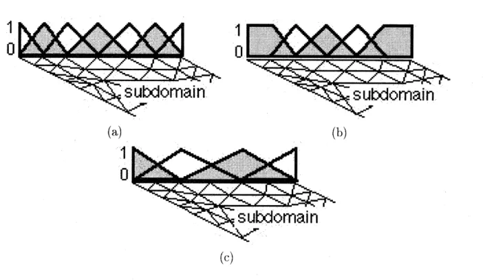
multiplier on the interfaces. For the discretization of the spaces of the Lagrange

multiplier defined on $\Gamma_{m}(1\leq m\leq M)$, we compare three cases (see Figure 2):

Case 1. The

conventional

iso-P2 Pl element, that is defined by

$W_{m,h}=(x_{\kappa(m)}+,h|_{\Gamma_{m}})^{2}$, (10)

where

$X_{k,h}=\{v\in C(\overline{\Omega_{k}}); v_{|e}\in P^{1}(e). e\in \mathcal{T}_{k./\iota/2}\}$ . (11)

Case 2. A modified iso-P2 Pl element having no freedorns at both edges of$\mathrm{i}\mathrm{n}\mathrm{t}\mathrm{e}\mathrm{r}\mathrm{f}\mathrm{a}\mathrm{C}\mathrm{C}\mathrm{S}[7]$.

Case 3. The

conventional

Pl element. that is defined by

(a) (b)

(c)

Figure 2: Shapes of (a)iso-P2, (b)modified iso-P2 and (c)P1 base functions for the

La-grarlge $\mathrm{m}\mathrm{u}\mathrm{l}\mathrm{t}\mathrm{i}_{1)}1\mathrm{i}\mathrm{e}\mathrm{r}$ and a sub$(\mathrm{l}\mathrm{i}\mathrm{V}\mathrm{i}\mathrm{s}\mathrm{i}\mathrm{o}\mathrm{n}\tau_{k,h/}2$

where

$Y_{k.h}.=\{v\in C(\overline{\Omega_{k}}); v_{1e}\in P^{1}(_{\mathrm{t}^{\supset}}’), e\in \mathcal{T}_{k,h}\}$. (13)

The finite elelnent, _space $W_{/\iota}$ is defined by

$\nu \mathrm{f}_{h}^{\Gamma}/=\prod_{m=1}^{M}\nu \mathrm{f}/rm,h$. (14)

We consider the time-discretized finite element equations derived from (1)$-(4)$

.

Problem 1. Find $(u_{h}^{n+\rfloor},l)hr?,$ $\lambda_{h}n)\in V_{h}\cross Q_{h}\cross 7\mathrm{t}_{h}^{\gamma}$, such that

$\forall v_{h}\in V’\iota,\backslash$ $( \frac{\prime(\iota_{h}^{n}+1-\prime l\mathit{4}_{h}^{\eta}}{\tau}, ?)h)_{h}+b(v_{hP_{h}}\backslash )\prime jn+(v_{h}, \lambda_{h}n)$ _$=$ $\langle\hat{f}, v_{h}\rangle$

$-a_{1}^{h}(u^{nn}, u_{h}, v_{h})h$

$-a_{0}(u_{h’ h}’‘)7\downarrow)\backslash$

, (15)

$\forall q_{h}\in Q_{h}$, $b(u^{n_{L}+},, qh)1$ $=$ $0$

.

(16) $\forall_{l}/_{h}\in W_{h}$, $j(u_{f_{1}}^{\eta+}, \mu_{h}1)$ $=$ $0$, (17)

where

$(u, v)$ $=$ $\sum_{k=1}^{I\backslash }-\int\Omega kuk$

.

$vkd_{\mathcal{T}}.$, (18)

$a_{1}(?r).u.\tau/))$ $=$ $\sum_{k=1}^{\tau_{\mathrm{i}}\prime}\int_{\Omega}k(w_{k}\cdot \mathrm{g}\mathrm{r}\mathrm{a}\mathfrak{c}1u_{k})v_{k}dX_{\backslash ,J}$ (19)

$a_{0}(u.?))$ $=$ $\frac{2}{Re}\sum_{k=1}^{Ic}\int\Omega ku_{k}D()\otimes D(v_{k})d_{X}.$

.

(20)

$b(v, q)$ $=$ $- \sum_{k=1}^{I\mathrm{t}’}\int\Omega kqk\mathrm{d}\mathrm{i}_{\mathrm{V}}vkdX$

.

(21)

$j(v, \mu)$ $=$ $- \sum_{m=1}^{M}\int \mathrm{r}mv_{\kappa}(+(m)-v(\kappa_{-}m))\mu_{m}ds$, (22)

$-\langle\hat{f}, v\rangle$

$=$ $\sum_{k=1}^{r}(\int I\mathfrak{i}\Omega_{k}f\cdot vkdx+\int_{\partial}\Omega_{k}\cap\Gamma_{N}^{\cdot}v_{k}gNd^{\sigma_{j}}.)$, (23)

$(, )_{h}$ denotes the mass-lumping corresponding to $($

.

$)$, $a_{1}^{h}$ is the upwind finite element

ap-proximation based on the choice ofup-and downwind $\mathrm{p}\mathrm{o}\mathrm{i}\mathrm{n}\mathrm{t}_{\mathrm{S}}[6]$ to

$\mathrm{c}x_{1},$ alld $D$ is the

$\mathrm{s}\mathrm{t}_{\mathrm{T}}\Gamma \mathrm{a}\mathrm{i}\mathrm{n}$

rate tensor.

We rewrite Problem 1 by a matrix form as,

$=$

,

(24)

where $\overline{M}$ is the lumped-mass $\mathrm{m}\mathrm{a}\mathrm{t}_{m}\mathrm{r}\mathrm{i}\mathrm{x},$ $B$ is the divergence matrix, $J$ is the jump matrix,

$F^{n}$ is a known vector, and $U^{n+1},P^{n}$ and $\Lambda^{n}$ are unknown vectors. Eliminating $U^{n+1}$

from (24), we get a domain-decomposition version of the consistent discretized pressure

$\mathrm{e}\mathrm{q}\mathrm{u}\mathrm{a}\mathrm{t}\mathrm{i}\mathrm{o}\mathrm{n}[8]$. Further eliminating $P^{n}$

.

we obtain a system of linear equations with respect

to $\Lambda^{n}$. Applying CG method to this equation. a domain decomposition algorithm is

obtained[9].

Remark 1. The quantity $\lambda_{m.h}$ corresponds to $\sigma\cdot n_{\kappa(m)}+|_{\gamma_{m}}$.

Remark 2. In implementation. an idea oftwo data$\mathrm{t}\mathrm{y}\mathrm{p}\mathrm{e}\mathrm{S}[10]$ is applied to the Lagrarlge

multipliers and the jump matrix. The idea simplifies the implementation and $\mathrm{r}\mathrm{e}(11\mathrm{l}\mathrm{c}\mathrm{e}$the

amount of message-passings. Forthe velocity and the pressure. we do not need to execute message-passlngs.

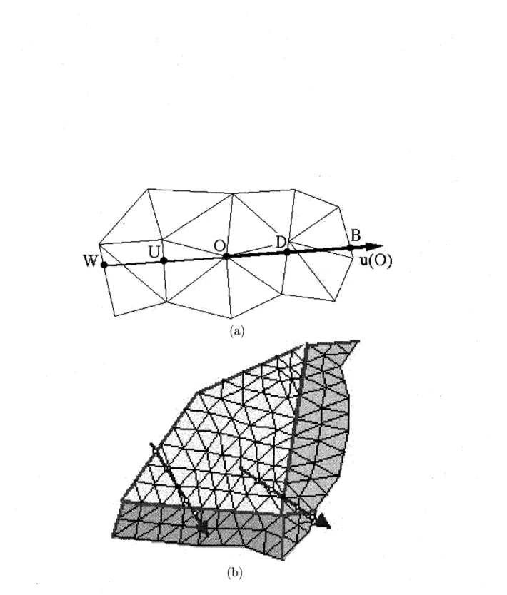
(b)

Figure 3: (a)Two upwind points(W,U) and two downwind points(D,B) in the upwind

finite element approximation based on the choice of up- and downwind $\mathrm{I}$)

$\mathrm{o}\mathrm{i}\mathrm{n}\mathrm{t}\mathrm{s}$ and

$(\mathrm{b})\mathrm{a}$

Remark 3. In order to evaluate $a_{1}^{h}(u^{\eta}u^{n}vh)h’ h^{\backslash }’$

’ we need to find two upwind $1$)

$\mathrm{o}\mathrm{i}\mathrm{n}\mathrm{t}\mathrm{s}$ and

two downwind points for each nodal points. In the $\mathrm{d}\mathrm{o}\mathrm{m}\mathrm{a}\mathrm{i}\mathrm{l}\mathrm{l}- \mathrm{C}\mathrm{l}\mathrm{e}\mathrm{C}^{\cdot}\mathrm{o}\mathrm{n}\mathrm{l}\mathrm{p}\mathrm{o}\mathrm{s}\mathrm{i}\mathrm{t}\mathrm{i}\mathrm{o}\mathrm{n}$situation. solne

of these up- and downwind points for nodal points near illterfaeies may be included in the

neighbor $\mathrm{s}\mathrm{u}\mathrm{b}\mathrm{e}1_{0}\mathrm{I}\mathrm{n}\mathrm{a}\mathrm{i}\mathrm{n}\mathrm{S}$. In order to treat it, each processor $\mathrm{c}\mathrm{o}\mathrm{r}\Gamma \mathrm{e}\mathrm{s}_{1\mathrm{g}}$)

$\mathrm{o}\mathrm{n}\mathrm{d}\mathrm{i}_{1\mathrm{l}}$ to a $\mathrm{s}\mathrm{u}\mathrm{t}$

)$(1_{0}\mathrm{n}\mathrm{l}\mathrm{a}\mathrm{i}_{11}$

has geornetry information of all elements which share at least a point with $\mathrm{n}\mathrm{e}\mathrm{i}\mathrm{g}\mathrm{h}\mathrm{t}$)$\mathrm{o}\mathrm{r}$

subdomains (see Figure $3(\mathrm{r}\mathrm{i}\mathrm{g}\mathrm{h}\mathrm{t})$). The processors exchange each other the values of $u_{h}^{r1}$

before the evaluation. Hence the evaluation itself is parallelized without any

message-passings.

3

Numerical

experiments

3.1

Test problem

Let $\Omega=(0,1)\cross(0,1)$ and $\Gamma_{D}=\partial\Omega(\Gamma_{N}=\emptyset)$ . The exact stational solution is

$u(x, y)$ $=$ $(x^{2}y+y^{3}, -x^{3}-xy2)^{T}$, (25)

$p(x, y)$ $=$ $x^{3}+y^{3}-1/2_{i}$ (26)

and the Reynolds number is set to 400. The boundary condition and the external force

are calculated from the stational Navier-Stokes equations.

We havedivided$\Omega$ into aunion of uniform $N\cross N\cross 2$triangularelements,where $N=4$,

8, 16 or 32. We have computed in two domain-decolnposed ways, where the number of

subdomains in each direction is 2 or 4. Figure 4 shows the domain-decomposition allcl the triangulation in the case $N=32$ and 4 $\cross 4$ subdomains. Starting from $\mathrm{a}\mathrm{r}\mathrm{l}$ initial

condition for the velocity, the numerical solution is expected to converge to the stational

solution in time-marching. If $\max_{k,i}|u_{k,i}^{n}-u^{n-1}k,i|/\tau<10^{-5}$ is satisfied. wejudge that the numerical solution has converged and stop the computation. Computation parameters

are set as $\tau=0.24/N$ and $\alpha=1.0$ (the latter is the stabilizing parameter of the upwind

approximation).

solu-Figure 4: Domain-clec($\mathrm{m}\mathrm{p}\mathrm{o}\mathrm{s}\mathrm{i}\mathrm{t}_{)}\mathrm{i}\mathrm{o}\mathrm{n}(4\cross 4)$ and the $\mathrm{t}\mathrm{r}\mathrm{i}\mathrm{a}\mathrm{n}\mathrm{g}\mathrm{u}\mathrm{l}\mathrm{a}\mathrm{t}\mathrm{i}_{0}\mathrm{n}(N=32)$

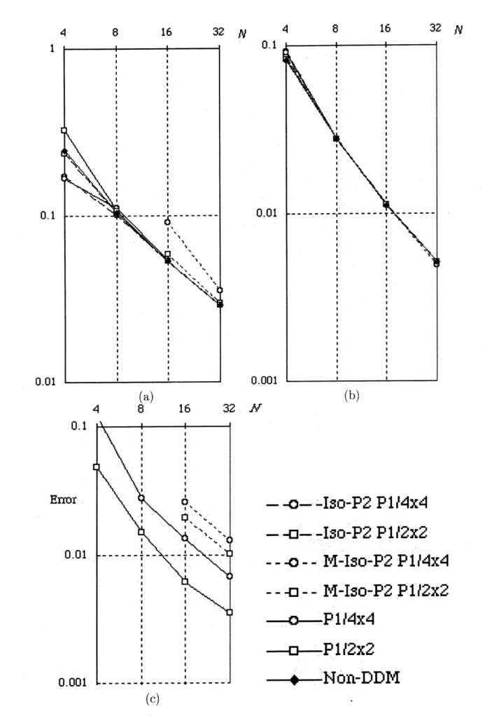
tions. They are measured by

$|v|_{V_{h}}= \{_{k=}I\sum_{1}’|v|^{2}(H1(\Omega_{k}))\backslash 2\}^{1/2}$, $||q||_{Q_{h}}= \{_{k=}I\sum_{1}’||q||_{L()}22\{\Omega_{k}\}^{1/2}$ ,

$|| \lambda||_{W_{h}}=\max_{rn\Gamma_{m}}\max|\lambda|$.

Results of the $\mathrm{n}\mathrm{o}\mathrm{I}1^{-}(1\mathrm{o}\mathrm{I}11\mathrm{a}\mathrm{i}\mathrm{n}-\mathrm{c}1_{\mathrm{C}\mathrm{C}\mathrm{O}\mathrm{I}}\mathrm{n}\mathrm{p}\mathrm{o}\mathrm{s}\mathrm{i}\mathrm{t}\mathrm{i}\mathrm{o}\mathrm{n}$ case are also plotted in the figure. We $\mathrm{c}\cdot \mathrm{a}\mathrm{l}\mathrm{l}$

observe $\mathrm{t}l\perp \mathrm{a}\mathrm{t}$ the

$\mathrm{e}\mathrm{r}\mathrm{l}\cdot \mathrm{o}\mathrm{r}\mathrm{s}$ of the velocity and the pressure realize the optimal convergence

rate of the iso-P2 $\mathrm{P}1/\mathrm{P}1$ elements,that is $O(h)$, regardless ofchoice of_{$W_{m,h}$}. In the first

case (iso-P2 Pl element for $W_{m,h}$), the maximum error of the Lagrange multiplier does

not converge to $0$ when $h$ tends to $0$

.

It may indicate the appearance of some spurious

Lagrallge multiplier modes, $\mathrm{s}\mathrm{i}11(i\mathrm{C}$ thedegree of freedom of the Lagrange$\mathrm{m}\mathrm{u}\mathrm{l}\mathrm{t}\mathrm{i}_{1}\mathrm{J}\mathrm{l}\mathrm{i}\mathrm{e}\mathrm{r}$ is larger

than that of jump of the velocity ill the choice. In the latter two cases the convergence of

the Lagrange multiplier has also observcd. The third case (Pl element for $\mathrm{w}\nearrow_{m,h}$) shows

the $\mathrm{t}$

)$\mathrm{e}\mathrm{s}\mathrm{t}_{1}1$)$\mathrm{r}\mathrm{o}\mathrm{P}(\mathrm{l}\mathrm{r}\mathrm{t}\mathrm{y}$ with $\mathrm{r}\mathrm{e}\mathrm{s}_{1^{\mathrm{J}\mathrm{e}\mathrm{c}\mathrm{t}}}$to the convergence of the Lagrange multiplier.

Since the ($j\mathrm{o}\mathrm{n}\mathrm{v}\mathrm{e}\mathrm{n}\mathrm{t}\mathrm{i}_{011\mathrm{a}1}$ Pl element has the smallest degree of freedom of the Lagrange

$\ln\iota 11\mathrm{t}\mathrm{i}_{1})1\mathrm{i}e\mathrm{r}$, it (an decrease the arlloullt of computation steps in a $\mathrm{i}\mathrm{t}\mathrm{e}\mathrm{r}\mathrm{a}\mathrm{t}\mathrm{i}_{0}11$ tinle ill $\mathrm{t}_{J}\mathrm{h}\mathrm{e}$

($\mathrm{o}\mathrm{n}\mathrm{j}_{1}1\mathrm{g}\mathrm{a}\mathrm{t}(^{>}\text{ノ}\mathrm{g}\mathrm{r}\mathrm{a}$(

$\mathrm{l}\mathrm{i}\mathrm{e}\mathrm{l}\mathrm{l}\mathrm{t}$ solver. Hence we adopt Pl element for

$\mathrm{M}^{I_{r}}$ in the $\mathrm{f}\mathrm{o}\mathrm{l}\mathrm{l}\mathrm{t}$

$N$

$–B–\mathrm{I}\mathrm{S}O- \mathrm{P}\Xi$

Pl

$f\triangleleft \mathrm{x}\mathrm{d}$

$– \mathrm{n}--\mathrm{I}\mathrm{s}o- \mathrm{p}\Xi$

Pl

$f\Xi \mathrm{x}\Xi$

–r–

$\mathrm{M}- \mathrm{I}\mathrm{s}o-\mathrm{P}\Xi$

Pl

$f\triangleleft \mathrm{x}\mathrm{d}$ $–\mathrm{f}\mathrm{i}--\mathrm{M}- \mathrm{I}\mathrm{S}o-\mathrm{P}\Xi$

Pl

$f\Xi \mathrm{x}\Xi$

(C)

1 $\cross 1$

1090.

3.2

Lid-driven cavity

flow problem

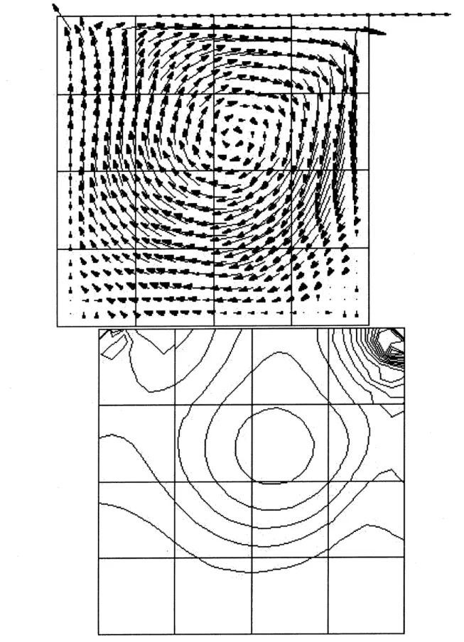
We next computed the two-dimensional lid-driven cavity flow problem. The Reynolds

number is 400. The domain $\Omega=(0,1)\cross(0,1)$ is divided into a uniform 24 $\cross 24\cross 2$

t,riangular subdivision. We chose $\tau=0.01$ and $\alpha=1$. We computed in the cases of$4\cross 4$,

4 $\mathrm{x}2,2\cross 2,2\cross 1$ and $1\cross 1$ domain-decompositions. The computation time are listed in

Table 1. We see that the ($.\mathrm{O}\ln_{\mathrm{P}^{\mathrm{u}\mathrm{t}}}\mathrm{a}\mathrm{t}\mathrm{i}\mathrm{o}\mathrm{n}$time becomes shorter as the number ofsubdomains

(i.e. processors) increases. $\mathrm{e}\mathrm{x}\mathrm{C}\mathrm{e}_{\mathrm{P}^{\mathrm{t}_{}\mathrm{f}}}\mathrm{o}1^{\cdot}$ the case of $2\cross 1$ subdomains. The velocity vectors

and the pressure colltours ofthe computed stationary fiow in $4\cross 4$ subdornains are shown

in Figure 6. We can observe that the flow is captured well in the dornain decomposition

algorithm.

4

Conclusion

Wehaveconsidered a domain decomposition algorithmofthe finiteelement scheme for the

Navier-Stokes equations. In the scheme, subdomain-wise finite element spaces by iso-P2

$\mathrm{P}1/\mathrm{P}1$ elernents are constructed and weak continuity of the velocity between subdomains are treated by a Lagrange multiplier method. This domain decomposition algorithm has

advantages such as: (i) each subdomain-wise problem is a consistent discretized pressure

Poisson equation so that it is regular, (ii) the size of a system of linear equations to be

solved by the conjugate gradient method is smaller than that of the original consistent

Figure

6:

Velocity vectors and pressurecontour lines of the lid-driven cavity flow problem,

Lagrange rnultiplier. $\mathrm{E}\mathrm{m}\mathrm{p}\mathrm{l}\mathrm{o}\mathrm{y}\mathrm{i}\mathrm{l}$ the conventional Pl element, we have computed $\mathrm{t}\mathrm{h}\mathrm{e}_{J}$

lid-driven cavity flow problem. $\mathrm{T}\}_{1}\mathrm{e}$ computation time becomes shorter when the number of

processor increases. We therefore recornmend iso-P2 Pl$(\prime u)/\mathrm{P}1(p)/\mathrm{P}1(\lambda)$ element in this

rnethod.

Acknowledgements

The author wish $\mathrm{t}_{\text{ノ}}()$ thank Professor Masahisa Tabata (Kyushu University) for many

valuable $\mathrm{c}\mathrm{l}\mathrm{i}\mathrm{s}\mathrm{c}\mathrm{u}\mathrm{s}\mathrm{S}\mathrm{i}\mathrm{o}\mathrm{l}\mathrm{l}\mathrm{s}\subset \mathrm{u}\mathrm{l}\mathrm{d}$ suggestions. The author was supported by the Ministry of

Ed-ucation, Science and Culture of Japan under Grant-in-Aid for Encouragement of Young

Scientists, No.09740148. The computations have been done on Intel Paragon $\mathrm{X}\mathrm{P}/\mathrm{S}$ in

INSAM($\mathrm{I}\mathrm{n}\mathrm{S}\mathrm{t}\mathrm{i}\mathrm{t}\mathrm{u}\mathrm{t}\mathrm{e}$ for $\mathrm{N}_{11\mathrm{m}\mathrm{e}}1^{\cdot}\mathrm{i}\mathrm{c}\mathrm{a}1$ Simulations and Applied Mathematics), Hiroshima

Uni-versity.

References

[1] Y. Achdou and Y. A. Kuznetsov. Algorithm for a non conforming domain

decompo-sition

rnethod.

Tcch. Rep. 296, Ecole Polytechnique.

1994.

[2] Y. Achdou andO. Pironneau, A fast solver forNavier-Stokes equations illthe lalninar

reginle using mortar finite element and boundary element methods, SIAM. J. Numer.

$Ar\iota al.,$ 32, 985-1016,

1995.

[3] R. Glowinski,T.-W. Pan and J. P\’eriaux. A one shot domain deconlposition/fi(titious

Scientific

and Engineering Computing, Proc. 7th Int.

_Conf.

on Domain

Decompo-$\dot{\Re}tion$, D. E. Keyes and J. Xu ($\mathrm{e}(1\mathrm{S}.)$, Contemporary Mathernatics 180., A. M. S.,

Providence. Rhode $\mathrm{I}\mathrm{s}\mathrm{l}\mathrm{a}\mathrm{n}\mathrm{d}_{J}\backslash$ 211-220,

1994.

[4] A. Suzuki, Implementation of donlain de($i\mathrm{o}\mathrm{m}_{1^{)\mathrm{o}\mathrm{s}}}\mathrm{i}\mathrm{t}\mathrm{i}\mathrm{o}\mathrm{n}$ methods on parallel

$(\mathrm{O}\mathrm{I}\mathrm{I}\mathrm{l}1^{)\mathrm{u}\mathrm{t}}\mathfrak{t}^{\backslash },\mathrm{r}$

ADENART. Parallel Computational Fluid Dynamics: New $Alg_{ori}thms$ and

Applica-tions, N. Satofuka, J. Periaux an(1 _{A. Ecer (eds.),} Elseviel.,

1995.

[5] M. Bercovier and O. Pironneau, Error estimates $\mathrm{f}\mathrm{o}1^{\cdot}$ finite element nletllo(1 solution

of the Stokes problem in the primitive variable, Numer. Math., 33.

211-224.

1979.

[6] M. Tabata and S. Fujima, An upwind finite element $\mathrm{s}\mathrm{c}\mathrm{h}\mathrm{e}\mathrm{l}\mathrm{n}\mathrm{e}^{\mathrm{Y}}$ for

high-Reynolds-number flows, Int. J. Num. Meth. Fluids, 12, 305-322, 1991.

[7] C. Bernardi, Y. Maday and A. Patera, A new nonconforming $\mathrm{a}_{1^{)}1^{)}}\mathrm{r}\mathrm{o}\mathrm{a}(i\mathrm{h}$ to clomaill

decomposition: the mortar element method., NonlinearPartial

Differential

Equation8

and their $Applicati_{\mathit{0}}n\mathit{8}\mathrm{x}\mathrm{I}$, H. Brezis and J. L. Lions (eds.). Longman

$\mathrm{S}(\mathrm{i}\mathrm{e}\mathrm{n}\mathrm{t}\mathrm{i}\mathrm{f}\mathrm{i}_{\mathrm{C}}\cdot$

&

Technical, Essex, UK, 13-51, 1994.

[8] P. M. Gresho, S. T. Chan, R. L. Lee allel C. D. Upson, A modified finite element

method for solving the $\mathrm{t}\mathrm{i}\mathrm{m}\mathrm{e}-\mathrm{d}\mathrm{e}_{1)\mathrm{e}}\mathrm{n}\mathrm{d}\mathrm{e}\mathrm{n}\mathrm{t}$, incompressible Navier-Stokesequations, Part

1: Theory, Int. J. Num. Meth. $Fluid_{\mathit{8}},4_{c}\backslash$ 557-598,

1984.

[9] S. Fujima, An upwind finite element scheme for the Navier-Stokes equations and its

domain decomposition algorithm, Thesis, Hiroshima University,

1997.

[10] S. Fujirna, Implementationof mortar element $1\mathrm{n}\mathrm{e}\mathrm{t}\mathrm{h}_{\mathrm{o}(}1$ for flow 1)roblems in the 1)$\mathrm{r}\mathrm{i}\mathrm{m}-$

itive variables, _{to appear in Int. J. Comp. Fluid Dyn.}

[11] S. Fujinla, Iso-P2 $\mathrm{P}1/\mathrm{P}1/\mathrm{P}\mathrm{l}\mathrm{D}\mathrm{o}\mathrm{m}\mathrm{a}\mathrm{i}\mathrm{n}- \mathrm{d}\mathrm{e}\mathrm{c}\mathrm{o}\mathrm{m}\mathrm{p}\mathrm{o}\mathrm{s}\mathrm{i}\mathrm{t}\mathrm{i}_{\mathrm{o}\mathrm{n}}/\mathrm{F}\mathrm{i}\mathrm{n}\mathrm{i}\mathrm{t}\mathrm{e}$-element Method for the