JAIST Repository: Program development in Java based on CafeOBJ specifications [課題研究報告書]

(1)

Japan Advanced Institute of Science and Technology

JAIST Repository

https://dspace.jaist.ac.jp/

Title Program development in Java based on CafeOBJ specifications [課題研究報告書]

Author(s) Ha, Xuan Linh Citation

Issue Date 2017-09

Type Thesis or Dissertation Text version author

URL http://hdl.handle.net/10119/14799 Rights

(2)

Program development in Java based on CafeOBJ

specifications

Ha Xuan Linh

School of Information Science

Japan Advanced Institute of Science and Technology

September, 2017

(3)

Master’s Project Report

Program development in Java based on CafeOBJ

specifications

1510214 Ha Xuan Linh

Supervisor : Professor Kazuhiro Ogata

Main Examiner : Professor Kazuhiro Ogata

Examiners : Professor Kunihiko Hiraishi

Professor Toshiaki Aoki

School of Information Science

Japan Advanced Institute of Science and Technology

(4)

Abstract

CafeOBJ is a powerful algebraic specification language that can be used for writing formal specifications of various software systems and verifying properties of them. It can be used as a powerful interactive theorem proving system. Despite its usefulness, up to present, few researches and engineers have used specifications written in CafeOBJ to develop soft-ware systems. Because most systems modeled in CafeOBJ are concurrent ones, we would like to propose methods or techniques that make it possible to write concurrent programs in Java based on observation transition systems (OTS) in CafeOBJ. In addition, we also propose a method to check if the concurrent program written in Java conforms to the OTS specification in CafeOBJ.

(5)

Acknowledgements

First of all, I would like to express my deepest appreciation to Professor Karuhiro Ogata, who gave me chance to join in his lab and supported me a lot not only in study but also in life during my Master program at JAIST.

I am grateful to my friends in the lab, who always help and share with me useful knowledge and funny experiences.

Lastly, I would like to say thanks to my family and many other friends who always encourage me to complete my study.

(6)

List of Figures

3.1 ABP . . . 19

4.1 State pattern in Java . . . 28

5.1 Programe design in Java . . . 35

5.2 State machine of the sender and receiver . . . 36

5.3 UML diagram of the sender and receiver . . . 37

5.4 State diagram of each PC . . . 39

5.5 UML diagram of each PC . . . 40

5.6 State diagram of each agent . . . 42

5.7 UML diagram of each agent . . . 42

(9)

List of Tables

2.1 Java and VDM++ types mapping . . . 15

3.1 Abstract Data Types for variables . . . 20

5.1 Type mapping in ABP simulator . . . 36

5.2 Type mapping in Simple Cloud . . . 39

(10)

Chapter 1 Introduction

In formal specification, two basic styles that are often used to formally specify a system are model-based and algebraic specification. In the model-based approach, the state of a system is represented by a set of data variables and transitions can be described by operations that manipulate these variables. All possible values of these variables, constrained by invariants over them define the state space of the system. Each operation is often defined with pre and post-conditions. This representation makes it likely easier for programmers to write programs as well as for automatic tools to generate codes in object-oriented programming languages from the specification. One of the well-known frameworks using this approach is VDM++ [5, 17], which has been applied to many industrial projects, such as the development of the "Mobile FeliCa" IC Chip Firmware, which is widely used in Japan [12]. While it is convenient to implement specifications written in VDM++, there is one issue that can be dealt with algebraic specification languages better than VDM++: formal verification. Some model-based specification languages, such as Z [21] and Event-B [9, 11], are equipped with a model checker and/or an interactive theorem prover, but to the best of our knowledge VDM++ is not. Testing is mainly used to check specifications written in VDM++.

In contrast, algebraic specification is more powerful in applying verification techniques [19, 20] but it seems more difficult for programmers to read and implement it. OTS is a way of specifying systems in algebraic approach, in which the semantics of the system is built from operators and axioms. In this report, we discuss how an OTS can be used to write concurrent programs in an object-oriented programming language. Java is selected in our projects because its concurrency features is powerful and there are also many useful testing frameworks in Java, which allows us to test the implementations, especially, Java PathFinder (JPF) [10]. This is a powerful model checker for Java bytecode programs, which can be applied to further check some properties of our implementations.

1.1 Motivation and Objectives

CafeOBJ is an advanced algebraic specification language that can be used for writing formal specifications of various software systems and verifying properties of them. It

(11)

im-plements equational logic by rewriting and can be used as a powerful interactive theorem proving system. Despite its usefulness, up to present, few researches and engineers have applied CafeOBJ specifications to software development, while object-oriented specifica-tion techniques such as VDM++, Event-B and Z are successfully applied to many projects. One of the reasons for the dominance of object-oriented approach is that specifications in this style are closer to program structures in imperative languages nowadays. Algebraic specification in CafeOBJ could bring significant advantages in verification but it may make more confuse for programmers to understand. The goal of this project is to reduce the gap between OTS specifications in CafeOBJ and the system implementations by proposing a technique to write a program based on its specification in CafeOBJ. Moreover, we discuss the method to test the written program based on its OTS specification.

1.2 Contributions

In this project we briefly introduce some specification techniques which have been success-fully applied to software development nowadays, the pros and cons of each technique and compare those techniques with CafeOBJ, an algebraic specification language currently used in our research group. In addition, we have proposed a possible way to write a concurrent Java program based on an OTS specification in CafeOBJ. By annotating the OTS specifications, programmers have more information about the concurrent programs they write such as the number of threads in the program, global and local variables and the methods in each thread. Because the systems specified in CafeOBJ are composed of several components interacting with each other, we have successfully applied state pattern in Java to design the programs where each component in the system can be developed as a separate state machine. This makes it easier for programmers to understand the pro-grams. Some case studies on writing the simulator of communication protocols such as ABP, Simple Cloud and Qlock are also represented in this research project to demonstrate our method.

Besides, we also propose a method to test the concurrent programs based on their OTS specifications by applying some external support tools such as JPF [10] and Maude [22]. JPF can model check Java bytecode programs but one of the most serious problem when using a model checker like JPF is the state space explosion where the size of the system state space grows exponentially as the number of state variables in the system increases. Despite of that, we could control JPF to model check a part of the whole state space. Maude is another model checker whose specifications can be converted from CafeOBJ specification by YAST [25, 26]. We intend to combine these two tools in our testing method to check if the written programs conform with the OTS specifications.

1.3 Thesis Outline

The outline of this report is as follows:

(12)

This chapter introduces the overview of formal specification methods nowadays and their application to software development. One of the most popular specification language for object-oriented designs, VDM++, is also represented in this chapter. Chapter 3: OTS Specification in CafeOBJ

This chapter discusses the features of OTS specifications in CafeOBJ. Chapter 4: Java and Design Patterns

This chapter talks about concurrent programming in Java and object-oriented design patterns that is commonly used in software development.

Chapter 5: Implementation Annotations in OTS Specifications and Case Studies

This chapter represents our techniques to write concurrent programs in Java based on OTS specifications in CafeOBJ. It discusses how annotations in the OTSs are used, the concurrent programs’ design and the mapping between components in OTS specifications and Java programs. This chapter also represents some case studies on writing the simulators of communication protocols based on their specifications. Chapter 6: Testing Concurrent Programs based on their OTS Specifica-tions

In this chapter we proposes a method to test the concurrent programs based on their specifications and some external support tools.

Chapter 7: Conclusion and Future Work This chapter concludes our project.

(13)

Chapter 2 Formal Specification in Software

Development

In this chapter, we represent the overview of formal specification methods nowadays and their applications to software development. In addition, we represent the features of one of the most popular formal specification language for object-oriented designs, VDM++, and its application to software development.

2.1 Overview of Formal Specification Methods

There are several research directions that are trying to apply formal specifications into software development process. In [6], a model-based approach to software specification in VDM++ is represented and the software’s codes can be automatically generated from those specifications. Specifications’ structures in VDM++ look like programs’ structure in Java. It includes many classes in which each system module is defined. State variables of a system are defined as attributes in Java classes with constrains on them. Operations in the systems are defined with pre and post conditions to make transitions in the model. The variable types in VDM++ are also similar to Java types such as Set, Queue, Map or others user defined data structures. VDM++ has used combinatorial testing where multiple test cases are generated from a given test expression to test its specification. While it is likely more straightforward to map a specification in VDM++ into Java codes compared with our technique but its model testing technique still has many limitations.

Event-B [1, 9, 11] is another research direction applying formal specification to software development. States of an Event-B model include constants and variables and the tran-sitions are declared as events, which are composed of guards and actions. Refinements in Event-B allow us to build models gradually until reaching the most refined one, which can be translated by hand or automatically into a real software. In order to support writ-ing Java programs based on Event-B models, [23, 4] have represented a tool - EB2Java - to translate models to JML annotated Java programs. Each event in a model can be translated into a subclass of Thread in Java in order to run in a multi-thread program or a standard Java class in a sequential one. The JML specification generated by EB2Java

(14)

can be used by programmers to checked against with their implementation by using avail-able JML tools [3]. The correctness of the final program is made sure by testing with JUnit test cases, which is manually written from an existing System Test Specification (STS) and proof obligations during each model refinement step. Our approach to testing concurrent programs written based on OTS specifications in CafeOBJ uses the rewrite theory specifications to which the OTS specifications are translated but do not use proofs (or proof scores) in CafeOBJ. We may want to investigate if it would be worth using proof scores in CafeOBJ to test such concurrent programs. If that is the case, we may consult the studies [23, 4].

Another paper [24] has proposed an automatic translation from OTS specifications in CafeOBJ into Java programs, but the generated Java programs are not concurrent ones. For one OTS, one Java class is generated in which observers and transitions are mapped to attributes and methods in the class.

The paper [18] proposes a way to generate test cases for invariant properties from proof scores for OTS specifications in CafeOBJ. Proof scores are proofs written in CafeOBJ. Test cases generated are dedicated to sequential programs and then cannot be used to test concurrent programs. If it is worth using proof scores to test our concurrent programs written based on OTS specifications, we may consult the work [18] even though the work is dedicated to sequential programs.

2.2 VDM++

VDM++ is an extension of VDM, a specification language for modeling object-oriented systems. In VDM, models are written in a flat manner, while in VDM++, they can be divided into many submodules and each module is described by a VDML++ class. This makes the structure of VDM++ models look similar to the one of Java programs. There are multiple parts in a VDM++ class such as types, instance variables, . . . as showed in Listing 2.1 and each part begins with a specific keyword. We will go through some important ones in a VDM++ class.

Listing 2.1: VDM++ structure class <class-name> types instance variables values operations functions traces thread sync end

2.2.1 Types

(15)

• bool : Boolean values.

• nat, nat1 : The nat type represents for natural number including 0 and nat1 is also used for natural numbers but it does not contain 0.

• int : Integer numbers. • real : Real numbers. • char : Character

• Quote type: This type is similar to enum type in Java. For example, we can define a type T like this: T = <France> | <Denmark> | <SouthAfrica>.

• Token type: Token type consists of a countably infinite set of distinct values, each value cannot be individually represented whereas they can be written with a mk_token. For example, mk_token(4), mk_token(5), mk_token(1, 2).

In addition, VDM++ also supports collection types such as set, sequence, map, . . . and user defined types and operations on them. For user defined types in VDM++, we can add the constraints to limit possible values of the type. For example, Listing 2.2 defines a Score type including multiple attributes and the last command defines a constraint on this type, a value of Score type is valid only if it satisfies this constraint.

Listing 2.2: VDM++ type constraint

Score :: team : Team won : nat drawn : nat lost : nat points : nat

inv_Score (sc) == sc.points = 3 * sc.won + sc.drawn;

2.2.2 Instance Variables

This part defines state variables of a VDM++ model and starts with instance variables keyword as showed in Listing 2.3.

Listing 2.3: VDM++ state variables

instance variables

public v1 : [int] := nil; public v2 : [int] := nil;

inv (v1 = nil or (-10 <= v1 and v1 <= 10))

The initial values of instance variables are assigned directly in the models and invariants on these variables can be declared after their definition. The last statement in Listing 2.3 is one of such invariants. Because instance variables may be changed by operations in the model, these constraints can be used for checking operations’ correctness.

(16)

2.2.3 Operations

Instance variables are updated by operators and all possible values of these variables together with the constrains on them define the state space of VDM++ models. There are two possible ways to define an operator in VDM++: explicit and implicit. While an explicit operator is defined with its body, an implicit operator is not. For example, Listing 2.4 defines an explicit operator to add an employee to a list of employees managed by the model and this operator can be redefined implicitly in 2.5. In the implicit version, the specification does not tell how the operation does.

Listing 2.4: VDM++ Explicit Operator

types

Id = token;

Detail :: name:seq of char age:nat1;

instance variables

employees: map Id to Detail := {|->}; operations

addEmployee : Id * Detail ==> ()

addEmployee(id,detail) == employees := employees munion {id |-> detail} pre id not in set dom employees

Listing 2.5: VDM++ Implicit Operator

types

Id = token;

Detail :: name:seq of char age:nat1;

instance variables

employees: map Id to Detail := {|->}; operations

addEmployee(id:Id, detail:Detail) pre id not in set dom employees

post exists id1 in set dom employees & id1=id and detail = employees(id)

An implicit operator is often defined with pre and post conditions. Pre-conditions must be satisfied in order to execute the operators and post-condition are required to be satisfied after the operator finishes.

2.2.4 Values and Functions

In VDM++ models, constants and functions are defined in values and functions parts respectively. Functions in VDM++ models are similar to operators but they cannot access or modify instance variables and they are often used by operators.

For concurrency models, thread and sync parts in the model are used but they are not mentioned in this report. Readers can refer to [13] for more details. Part traces is used for model testing and we will discuss about it in the next section.

(17)

2.3 Model Testing in VDM++

One of the most useful features in VDM++ is the application of combinatorial testing [13, 14] to test models. Instead of manually writing test cases for sequence of operators in the models, test cases are automatically generated from expression defined in traces part. Let us take an example to see how combinatorial testing are used in VDM++. Supposed that a VDM++ model has two operators loadTable and swap as defined in Listing 2.6, where the type table is a map from string to natural number and student type is equivalent with string:

Listing 2.6: Operators for combinatoral testing

loadTable : table ==> ()

swap : student * student ==> ()

The loadTable operator takes a map from string to natural number as an input and stores to an instance variable. swap operator receives two string and exchange two values in the map. Now we want to check if there is any error when a sequence of operators is executed. In manual manner, we could write test cases one by one as showed in Listing 2.7. There are some errors that is difficult to find out if we do not have enough test cases.

Listing 2.7: One possible test case for VDM++ model

Trace1 : loadTable({"a"|->1,"b"|->1,"c"|->1,"d"|->1,"e"|->2,"f"|->2,"g "|->2});

swap("a","b"); swap("a","e"); swap("a","a");

Therefore, VDM++ allows us to write testing expression to automatically generate as many test cases as possible. Listing 2.8 shows an example testing expression.

Listing 2.8: Testing expression in VDM++ model

Trace2 : loadTable({"a"|->1,"b"|->1,"c"|->1,"d"|->1,"e"|->2,"f"|->2,"g "|->2});

(let x in set {"a", "f"} in

let y in set {"a", "b", "e", "f"} in swap(x,y)){1,2};

In the testing expression, variable x takes possible values from the set {"a", "f "} and y takes values from the set {"a", "b", "e", "f "} to form parameters of swap operator. The notation {1, 2} after swap(x,y) indicates that this operator can be executed one or two times. Therefore, there are total 72 possible test cases generated from this expression. Although this feature can save labor for user but it may slow down the performance to test all possible test cases. For that reason, combinatorial testing in VDM++ allows us skip unnecessary test cases when they are covered by previous ones and filter specific test cases to be tested on the models based on a specific condition from users.

(18)

2.4 Translating VDM++ to Java

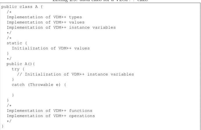
Because the structure of VMD++ models are similar to Java classes, the conversion from VDM++ to Java program is pretty straightforward. There are many translation tools developed by different research groups and here we introduce one from [2] where each VMD++ class is translated into a Java class whose general structure is represented in Listing 2.9.

Listing 2.9: Java class for a VDM++ class

public class A { /*

Implementation of VDM++ types Implementation of VDM++ values

Implementation of VDM++ instance variables */ /* static { Initialization of VDM++ values } */ public A(){ try {

// Initialization of VDM++ instance variables } catch (Throwable e) { } } /* Implementation of VDM++ functions Implementation of VDM++ operations */ }

Most VDM++ types can be successfully converted into Java classes and the mapping between them is showed in Table 2.1. Each quote type in VDM++ is translated into a Java class.

VDM++ Type Java Type

real, rat Double

nat, nat1, int Integer

bool Boolean

char Character

seq Vector

map HashMap

Table 2.1: Java and VDM++ types mapping

(19)

attributes in the Java class respectively. Java codes generated in the constructor will initialize values of attributes and this comes from the initialization of instance variables in VDM++. Operators and functions will be translated into methods in Java class.

Multiple inheritance is allowed in VDM++ but it is not in Java. Although Java does not allow multiple inheritance, a Java class can implement multiple interfaces. Therefore, in order to successfully translate multiple inheritance in VDM++ into Java classes, there must be some additional requirements. The first requirement is that only one supper class may define function and operation implementations and only this superclass may provide instance variables. This class will be generated as the single superclass in Java and secondly, other super classes in VDM++ must be possible to be translated into interfaces.

(20)

Chapter 3 OTS in CafeOBJ

In this chapter, we discuss some basic concepts in algebraic specification and the OTS method in CafeOBJ. One example OTS specification is also represented in this chapter.

3.1 Data

Data in CafeOBJ are represented by sorts. A sort is used to denote a set and corresponds to a type in programming languages. The set denoted by a sort is composed of a same sort of elements (or values) that are represented by operators called constructors. Operators are also used to represent functions, which are defined in terms of equations. For example, Listing 3.1 is a specification of natural numbers:

Listing 3.1: Specification of natural numbers

mod! PNAT { [Nat]

op 0 : -> Nat {constr} . op s_ : Nat -> Nat {constr} . op _+_ : Nat Nat -> Nat . vars X Y : Nat .

eq 0 + Y = Y .

eq s(X) + Y = s(X + Y) . }

Basic units of specifications in CafeOBJ are modules. PNAT is a module in which natural numbers are specified. The sort Nat denotes the set of natural numbers. The operators 0 and s are the constructors of natural numbers, which are constructed from 0 and s, such as 0, s(0), s(s(0)) and s(s(s(0))). The operator _ + _ is used to denote the addition of natural numbers, which is defined with the two equations, where X and Y are variables of Nat. Equations are used as left-to-right rewrite rules to reduce terms. For example, s(s(s(0))) + s(s(s(s(0)))) reduces to s(s(s(s(s(s(s(0))))))) by using the second equation three times and the first equation once.

In an OTS specification, there is a special sort that denotes the set of reachable states. Hereafter, we use Sys as the special sort. In an OTS specification, each state is charac-terized by values called observable values. Observable values are observed by operators

(21)

called observers. State transitions are represented by operators called transitions. How to change observable values by state transitions are defined in terms of equations. We will describe observers and transitions.

3.2 Observers

Observers in an OTS are operators that are used to extract values that characterize states of the OTS. An observer takes one state and zero or more data values and returns a data value. For example, if one natural number and one Boolean value fully characterize each state of an OTS, it suffices to have two observers in Listing 3.2:

Listing 3.2: Observers in an OTS

mod* SYS { pr(PNAT) [Sys] op o1 : Sys -> Nat . op o2 : Sys -> Bool . ... }

pr(PNAT) imports PNAT module declared in Listing 3.1. Observer o1 takes one state and returns a natural number and observer o2 takes one state and returns one Boolean value.

3.3 Transitions

Transitions in an OTS are operators that are used to represent state transitions. A transition takes one state and zero or more data values and returns a state, where the latter is a successor state of the former. Transitions are defined in terms of equations that describe how to change observable values in a successor state from a given state with respect to a transition. For example, we have two transitions trans1 and trans2 in Listing 3.3 as follows:

Listing 3.3: Transitions in an OTS

mod* SYS { pr(PNAT) [Sys]

op o1 : Sys -> Nat . op o2 : Sys -> Bool . op trans1 : Sys -> Sys . op trans2 : Sys -> Sys .

ceq o1(trans1(S:Sys)) = o1(S) + s(0) if o2(S) . ceq o2(trans1(S:Sys)) = o2(S) if o2(S) .

ceq trans1(S:Sys) = S if not o2(S) . eq o1(trans2(S:Sys)) = 0 .

eq o2(trans2(S:Sys)) = not o2(S) . }

(22)

The transition trans1 has the condition that the Boolean value is true in a given state, while trans2 does not. The first equation says that the natural number is increased in the successor state denoted as trans1(S:Sys) if o2(S) is true, where S is a variable of Sys. Variables can be declared before equations or on-the-fly in equations. The second equation says that the Boolean value does not change with trans1. The third equation says that nothing changes with trans1 if the condition does hold in a given state. The first three equations define trans1. The fourth equation says that the natural number becomes zero with trans2, and the fifth equation says that the Boolean value is toggled with trans2. The last two equations define trans2.

3.4 Sample OTS: ABP specification

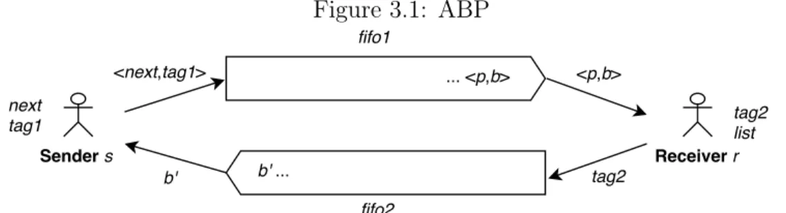
In order to have a better understanding of OTS specification, in this section, we repre-sent a detail specification of a communication protocol. ABP has been selected for this demonstration. This is a protocol used for sending a sequence of packages from a sender to a receiver over unreliable channels as showed in Figure 3.1. The sender s keeps two

Figure 3.1: ABP

information including the next package to be sent and a boolean value tag1 and the sender keeps a list to store received packages and a boolean value tag2. There are two unreliable channels between the sender and receiver called fifo1 and fifo2. Initial values of both tag1 and tag2 are true. Whenever the sender receives a boolean value from channel fifo2, it checks if this received value is different from its current tag1 value. If that is the case, the sender negates flag1 and prepare the new package by increasing next by 1; otherwise, the received boolean value from fifo2 will be discarded. On the other side, whenever the receiver gets a pair of package number and boolean value from channel fifo1, it checks if the boolean value is the same as flag2. If they are the same, the receiver negates flag2 and store the package number to the list ; otherwise, it discards the pair. The two chan-nels fifo1 and fifo2 are unreliable and their packages may be dropped or duplicated. For simplicity, we supposed that drop or duplication occur only with the top package of each channel. ABP makes sure that the receiver eventually receives correct sequence of data from the sender.

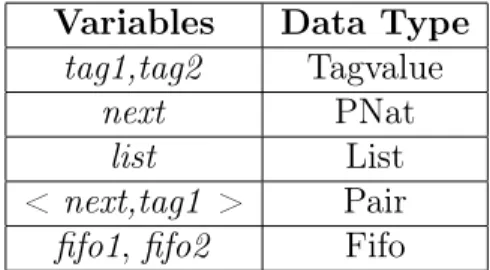
In the specification, we need abstract data types to represent variables in the system and Table 3.1 shows each variables’ data types:

(23)

Variables Data Type tag1,tag2 Tagvalue

next PNat

list List

< next,tag1 > Pair fifo1, fifo2 Fifo

Table 3.1: Abstract Data Types for variables

Each data type is defined in a separated module and we look at the detail each of them. The first one is Tagvalue, which is represented in Listing 3.4.

Listing 3.4: Tagvalue data type in CafeOBJ

mod! TAGVALUE { [Tagvalue]

ops up down : -> Tagvalue op flip : Tagvalue -> Tagvalue

op _=_ : Tagvalue Tagvalue -> Bool {comm} var V : Tagvalue

eq flip(up) = down . eq flip(down) = up . eq (V = V) = true . eq (up = down) = false . eq (flip(V) = V) = false . }

Two operators up and down can be seen as two constants of Tagvalue sort. The flip operator is defined to toggle a variable of this data type and _=_ operator is used to identify equality of two values of this type.

The definition of PNat data type is already showed in Listing 3.1, so we do not represent it here again. The definition of List data type is showed in Listing 3.5.

Listing 3.5: List data type in CafeOBJ

mod! LIST { pr(PNAT) [List]

op nil : -> List

op __ : Nat List -> List op hd : List -> Nat op tl : List -> List op mk : Nat -> List

op _=_ : List List -> Bool {comm} vars L L1 L2 : List vars X Y : Nat eq hd(X L) = X . eq tl(X L) = L . eq mk(0) = 0 nil . eq mk(s(X)) = s(X) mk(X) . eq (L = L) = true .

(24)

eq (nil = nil) = true . eq (nil = X L) = false .

eq (X L1 = Y L2) = (X = Y and L1 = L2) . }

The first two operators in LIST module can be called constructor operators because all possible values of List data type can be represented by these two operators. Others are necessary operators on List data type such as taking the first element, getting the tail or making a list of natural number from zero to a specific value.

Next, we go to Pair data type defined in PAIR module in Listing 3.6. Listing 3.6: Pair data type in CafeOBJ

mod* EQTRIV { [Elt]

op _=_ : Elt Elt -> Bool {comm} }

mod! PAIR(D1 :: EQTRIV, D2 :: EQTRIV) principal-sort Pair { [Pair]

op <_,_> : Elt.D1 Elt.D2 -> Pair op 1st : Pair -> Elt.D1

op 2nd : Pair -> Elt.D2

op _=_ : Pair Pair -> Bool {comm} var X : Elt.D1 var Y : Elt.D2 vars P P1 P2 : Pair eq 1st(< X , Y >) = X . eq 2nd(< X , Y >) = Y . eq (P = P) = true . eq (P1 = P2) = (1st(P1) = 1st(P2) and 2nd(P1) = 2nd(P2)) . }

PAIR is a parameterized module where D1 and D2 can be seen as two module parameters. Elt.D1 denotes a sort in parameter module D1. The first operator in the PAIR module defines the structure of each element in Pair, also called constructor, while others are defined to handle values of this type such as taking the first or the second value of a pair. The Queue data type with supporting operations are defined in Listing 3.7. This is also a parameterized module.

Listing 3.7: Fifo data type in CafeOBJ

mod! FIFO(D :: EQTRIV) { [Fifo]

-- data constructors op empty : -> Fifo

op _|_ : Elt.D Fifo -> Fifo -- operators

op put : Fifo Elt.D -> Fifo op get : Fifo -> Fifo

op top : Fifo -> Elt.D op empty? : Fifo -> Bool op _\in_ : Elt.D Fifo -> Bool

(25)

op _=_ : Fifo Fifo -> Bool {comm}

op _@_ : Fifo Fifo -> Fifo -- concatenate two fifos op del : Fifo -> Fifo -- delete the last element --vars X Y Z : Elt.D vars F F1 F2 : Fifo eq put(empty,X) = X | empty . eq put((Y | F),X) = Y | put(F,X) . eq get(X | F) = F . eq top(X | F) = X . eq empty?(empty) = true . eq empty?(X | F) = false . eq X \in empty = false .

eq del(X | empty) = empty .

eq del(X | Y | F) = X | del(Y | F) .

eq del(F1 @ (X | F2)) = F1 @ del(X | F2) .

--ceq X \in put(F,Y) = true if X \in F or X = Y . ceq X \in put(F,Y) = false if not(X \in F or X = Y) . eq put(F1 @ F2,X) = F1 @ put(F2,X) .

eq empty?(F1 @ F2) = empty?(F1) and empty?(F2) .

eq (empty = (F1 @ F2)) = (empty = F1) and (empty = F2) . eq ((Z | empty) = (F1 @ (X | Y | F2))) = false .

}

As the comments starting with "--" in the specification, two operators empty and _|_ are constructors of this data type. Others are necessary operators related to a queue structure such as putting the end of a queue, get the top of a queue and so on.

After defining necessary data types, let us look at the specification of ABP. In general, there are two main parts in an OTS specification: observers and transitions. Looking at the Listing 3.8, there are six observers and eight transitions in ABP’s OTS specification.

Listing 3.8: Obervers and transitions in ABP specification

-- observers

bop fifo1 : System -> PFifo -- Sender to Receiver channel bop fifo2 : System -> BFifo -- Receiver to Sender channel bop tag1 : System -> Tagvalue -- Sender’s tag

bop tag2 : System -> Tagvalue -- Receiver’s tag

bop next : System -> Nat -- the number Sender wants to deliver bop list : System -> List -- the numbers received by Receiver -- actions

bop send1 : System -> System -- Sender’s sending numbers bop rec1 : System -> System -- Sender’s receiving acks

(26)

bop send2 : System -> System -- Receiver’s sending acks bop rec2 : System -> System -- Receiver’s receiving numbers bop drop1 : System -> System -- drop the 1st of fifo1

bop dup1 : System -> System -- duplicate the 1st of fifo1 bop drop2 : System -> System -- drop the 1st of fifo2 bop dup2 : System -> System -- duplicate the 1st of fifo2

A transition in an OTS is defined by the change of observers after it is successfully executed. For example, rec1 transition is defined in Listing 3.9 through the change of fifo1 observer. Because this transition only changes the value of fifo1, others observer values are unchanged after this transition finishes.

Listing 3.9: Behavior specification of ABP

var S : System

-- for initial state eq fifo1(init) = empty . eq fifo2(init) = empty . eq tag1(init) = up . eq tag2(init) = up . eq next(init) = 0 . eq list(init) = nil . -- send1

eq fifo1(send1(S)) = put(fifo1(S),< tag1(S) , next(S) >) . eq fifo2(send1(S)) = fifo2(S) . eq tag1(send1(S)) = tag1(S) . eq tag2(send1(S)) = tag2(S) . eq next(send1(S)) = next(S) . eq list(send1(S)) = list(S) . -- rec1

op c-rec1 : System -> Bool {strat: (0 1)} eq c-rec1(S) = not empty?(fifo2(S)) .

--eq fifo1(rec1(S)) = fifo1(S) .

ceq fifo2(rec1(S)) = get(fifo2(S)) if c-rec1(S) . ceq tag1(rec1(S))

= (if tag1(S) = top(fifo2(S)) then tag1(S) else top(fifo2(S)) fi) if c-rec1(S) .

eq tag2(rec1(S)) = tag2(S) . ceq next(rec1(S))

= (if tag1(S) = top(fifo2(S)) then next(S) else s(next(S)) fi) if c-rec1(S) .

eq list(rec1(S)) = list(S) .

ceq rec1(S) = S if not c-rec1(S) .

One transition often goes with a condition. For example, rec1 transition is defined with one additional condition, c-rec1. It says that the transition is enabled to execute only if its condition is satisfied. Initial observer values of an OTS are also defined as the top of Listing 3.9. These definitions let reader know the values of system’s variable at the beginning.

(27)

Chapter 4 Concurrent Programming in Java and

Design Patterns

4.1 Concurrent Programming in Java

Because Java is a commonly used programming language, we are not going to write details about the language. Here, we just introduce some important features to write a concurrent program in Java. Besides, we also mention design patterns that are commonly used for software designs in Java.

4.1.1 Threads

A concurrent program in Java includes multiple threads and there are two possible ways to define the code that will run in each thread. The first way is to define a class that implements Runnable interface as the Listing 4.1.

Listing 4.1: Defining a thread by implementing Runnable interface public class Sender implements Runnable {

// ...

public void run() {

// TODO: thread will run code here }

// ...

public static void main(String args[]) { (new Thread(new Sender())).start(); }

// ... }

In order to create a new thread, we need to pass an object of Runnable type to Thread ’s constructor and call start method of Thread. After the statement (new Thread(new Sender())).start(); in Listing 4.1 is executed, a new thread is created and runs what is defined inside the run method.

(28)

Listing 4.2: Defining a subclass of Thread public class Sender extends Thread {

// ...

// TODO: thread will run code here }

// ...

public static void main(String args[]) { (new Sender()).start();

} // ... }

In this way, the new class inherits Thread and we just call start method from an instance of this subclass to initiate a new thread. Similar to the first way, the new thread created will runs what is defined inside the run method.

4.1.2 Synchronization

In a concurrent program, threads may interact with each other and this can cause errors if we do not have appropriate policies to control them. If multiple threads try to access the same resource simultaneously without any synchronization, memory consistency errors may happen. For example, the Listing 4.3 shows an erroneous multi-thread program in Java because there is no synchronization between threads.

Listing 4.3: Errors in multi-thread program class Counter{

private int c = 0;

public void increment() { c++;

}

public void decrement() { c--;

}

public int getValue() {

return c; }

}

public class UnsafeInc extends Thread {

private static final int LOOPS = 1000;

private Counter c;

public UnsafeInc(Counter c) {

this.c = c; }

for (int i = 0; i < LOOPS; i++) { c.increment();

} }

(29)

Counter c = new Counter();

UnsafeInc t1 = new UnsafeInc(c); UnsafeInc t2 = new UnsafeInc(c); t1.start(); t2.start();

t1.join(); t2.join();

System.out.println(c.getValue()); }

}

There are two threads initiated in the above program to increase a counter value. Each thread increases the counter 1000 times, therefore, in theory, the final counter value should be 2000. But the actual value we get can be less than 2000. The reason is that the statement c++; is not atomic. This means that c++; can be decomposed into smaller steps. We do look at deeper into bytecode instructions generated for c++; but in general, it can be decomposed into three steps:

• Retrieve the current value of c. • Increment the retrieved value by 1. • Store the incremented value back in c.

The two thread may interleave these three steps and this causes the final result different from what is expected.

The mechanism Java provides to prevent these kinds of error is called synchronization. There are two levels of synchronization in Java: method synchronization and statement synchronization. We will explain each of them. The Listing 4.4 shows a new counter whose all methods are defined with synchronized keyword.

Listing 4.4: Method Synchronization public class SynchronizationCounter {

public synchronized void increment() { c++;

}

public synchronized void decrement() { c--;

}

public synchronized int getValue() {

return c; }

}

Supposed that counter is an object of SynchronizationCounter class, if the synchronization methods of counter are called by different threads, all statements inside the method will be executed atomically. If we do not want to synchronize the whole method, we use statement synchronization to synchronize a particular block of statements, this can make the concurrent applications’ performance better in case that the method contains a long sequence of statements. For example, in the Listing 4.5, because we want all thread synchronize on c++; statement, we need to put it inside a synchronization block.

(30)

Listing 4.5: Method Synchronization public class StatementSynchronization {

public void exampleMethod() { // more things to do synchronized (this) { c++; } // more things to do } }

If sc is an object of StatementSynchronization class and there are multiple calls to exampleMethod of sc, then only one statement c++; is executed atomically while other can be run simultaneously by multiple threads.

In Java, there is a lock associated with each object and if a thread acquires the lock of the object that is passed to the synchronization block, other threads must wait the first thread’s finish to acquire the lock to run the synchronized statement block. A synchronized method can be rewritten using statement synchronization by wrapping all statements inside the method into a synchronization block and pass this as the parameter of the synchronization block.

4.2 Design Patterns

In order to have a good software design, we should follow some principles based on the feature of the language we use. Because Java is an object-oriented programming lan-guage, there are some strategies to write software in this language called object-oriented design patterns. If these patterns are applied appropriately to software development, the softwares become easier to manage, develop and modify if there are changes in require-ments. These strategies often take advantage of features in object oriented programming language such as inheritance, polymorphism and rely on criteria such as separability of software components. In this section, we introduce some design patterns in Java that can be used in this research project. If readers want to take a deeper understanding about design patterns, please refer to [7].

4.2.1 Singleton design pattern

This pattern is one of the simplest design patterns in Java. The intent of this pattern is to ensure that a class has only one instance and provides a global access to it. The code in Listing 4.6 is one of the common ways to define a singleton class in Java.

Listing 4.6: Singleton class in Java public class Singleton {

private Singleton instance; // TODO: define attributes

(31)

// TODO: initialization }

public Singleton getInstance() {

if (instance != null) {

instance = new Singleton(); }

return instance; }

// TODO: define other public methods }

In Singleton class, an instance of this class is defined and its constructor goes with private acccess modifiers to insure that object creation cannot be done outside the class. A method called getInstance provides access to this unique instance inside the class and this instance is lazy-initialized, that means it is initialized only when it is needed. All of other public methods are accessed via this method.

4.2.2 State Design Pattern

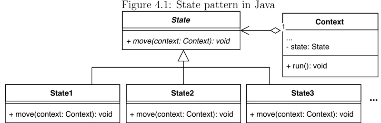
This pattern is often used to represent an state machine in Java. This pattern can be visualized in Fig. 4.1. An instance of Context class can be viewed as a state machine in a

Figure 4.1: State pattern in Java

program. The data of a state machine is stored in Context class and possible states of the machine are represented by concrete subclasses of State. There is one abstract method move in State class and it is implemented differently by subclasses.

We write a simple program to represent the state machine of a light to illustrate this design pattern. A light has two possible states: On and Off and the switch method is responsible for switching its current state. Listing 4.7 shows the definition of Light class. Light class keeps a state attribute and each time a light receives a switch message, it calls the move method on its state. Possible states of a light are represented by Java classes in Listing 4.8.

Listing 4.7: Light class public class Light {

(32)

public Light() {

super();

this.state = new StateOff(); }

public void swith() { state.move(this); }

public State getState() {

return state; }

public void setState(State state) {

this.state = state; }

}

Listing 4.8: Possible states of a light public abstract class State {

public abstract void move(Light light); }

public class StateOff extends State { @Override

public void move(Light light) { State state = new StateOn(); light.setState(state);

System.out.println("Now is On!"); }

}

public class StateOn extends State { @Override

public void move(Light light) { State state = new StateOff(); light.setState(state);

System.out.println("Now is Off!"); }

}

In order to see how a light works, we define a Main class in Listing 4.9. The Main class creates a light and sends switch message to the light two times.

Listing 4.9: Main class public class Main {

public static void main(String[] args){ Light light = new Light();

light.swith(); light.swith(); }

}

(33)

Now is On! Now is Off!

Each time a switch message is sent to the light, it switches its state and prints out the new one. Because the light’s initial state is Off, then the sequence of states printed out are On and Off.

4.2.3 MVC Design Pattern

Another design pattern that is often used in software development is MVC. The goal of this pattern is to separate an application’s components based on its functionality:

• Model: Models are POJO Java classes carrying data of the application. • View: View is responsible for visualizing the data contained in model.

• Controller: Controller operates on both model and view. It can modify data in the model and update the view whenever model is changed.

Let us see an example application to manage employees in a company. Here the data that need to be managed are employees and each of them is represented by Employee class as showed Listing 4.10.

Listing 4.10: Employee model public class Employee {

private int id;

private String name;

public Employee(int id, String name) {

this.id = id;

this.name = name; }

public String toString() {

return "[ ID:" + id + ", Name: " + name + "]"; }

}

The view is represented by EmpView class in Listing 4.11. It simply prints out the list of employees in order.

Listing 4.11: Employee view public class Employee {

private int id;

private String name;

public Employee(int id, String name) {

this.id = id;

this.name = name; }

public String toString() {

return "[ ID:" + id + ", Name: " + name + "]"; }

(34)

Finally, the employee controller containing references to the model and view is illus-trated in Listing 4.12.

Listing 4.12: Employees controller public class EmpController {

private List<Employee> es;

private EmpView ev;

public EmpController(List<Employee> es, EmpView ev) {

this.es = es;

this.ev = ev; }

public void modEmp(Employee e) {

boolean isUpdate = false;

for (Employee e1 : es) {

if (e1.getId() == e.getId()) { e1.setName(e.getName()); isUpdate = true; } } if (!isUpdate) { es.add(e); } }

public void rmEmp(int id) {

for (int i = 0; i < es.size(); i++) {

if (es.get(i).getId() == id) { es.remove(i); break; } } }

public void updateView() { ev.dispEmps(es);

} }

It allows external components to modify models by two methods modEmp and rmEmp and to update the view by updateView method. The demo application in Listing 4.13 illustrates how this pattern is used.

Listing 4.13: Demo application of MVC pattern public class Demo {

public static void main(String[] args) { List<Employee> es = getEmployees(); EmpView ev = new EmpView();

EmpController ec = new EmpController(es, ev); ec.updateView();

// modify and display

ec.modEmp(new Employee(23, "John")); ec.updateView();

// remove and display ec.rmEmp(35);

(35)

ec.updateView(); }

private static List<Employee> getEmployees() { List<Employee> es = new ArrayList<Employee>(); es.add(new Employee(23, "Peter"));

es.add(new Employee(35, "Marry"));

return es; }

}

Result:

0: [ ID:23, Name: Peter] 1: [ ID:35, Name: Marry] 0: [ ID:23, Name: John] 1: [ ID:35, Name: Marry] 0: [ ID:23, Name: John]

Each time the model is changed via the controller ec and the view is updated, we get a different result. Here the controller is the main access point to the model and view. MVC is often used in web development frameworks where model is usually stored in a database, the view is responsible for generating a specific html view for data and the controller is responsible for receiving and processing requests from users via the forms on the view or via ajax calls.

There are many other useful patterns that reader can find in [7] and because this are not the main topic of this project, we just briefly introduce some of them. In this research project, we apply state pattern to implement our concurrent programs because most system modeled in OTS are composed of many state machines interacting with each other and each of them can be designed by this pattern.

(36)

Chapter 5 Implementation Annotations in OTS

Specifications and Case Studies

In this section, we propose steps to write a concurrent program in Java programming language based on an OTS specification in CafeOBJ and show some case studies for the method.

5.1 Implementation Annotations in OTS Specifications

In this section, we propose steps to write a concurrent program in Java programming language based on an OTS specification in CafeOBJ. However, programmers need to infer several non-trivial things from OTS specifications. To mitigate the issue, therefore, we also propose annotations to implement OTS specifications as concurrent programs. Annotations are written in OTS specifications as CafeOBJ comments.

5.1.1 Step1: Identifying threads in the program

Because the program we write is concurrent, we firstly need to identify threads running in the program. They are considered as entities which are able to change the system state. In some OTSs, transition operators contain information about which entity execute those transitions, then we can infer threads’ information in the concurrent program but in general cases, this requires implementors to have some understandings of the system. For this reason, we use comments in the specification to identify threads in the program.

Listing 5.1: Threads in a concurrent program

mod* ABP {

-- #IMP: Threads: Sender, Receiver, DropDuplicator [Sys]

-- any initial state op init : -> Sys -- observers ...

(37)

... }

The comments starting with "-- #IMP:" will be used by implementors. For example, from the first comment of ABP’s specification in the Listing 5.1, programmers know that there are three threads called "Sender", "Receiver" and "DropDuplicator" running in the concurrent program they need to implement.

5.1.2 Step2: Mapping of observers and transitions

The set of observers in an OTS can be seen as the set of data variables in model-based specifications such as VDM++. The difference is that by looking at observers in an OTS, we do not know which ones belong to which thread and which ones are global in the concurrent program. Therefore, programmers need to understand the system to distribute observers to correct place in the program. To deal with this issue, we also use comments in the specification as directives for programmers. So, by looking at the comment before each observer, we map it to attributes of the correct thread. The type of each variable in Java program must be correctly chosen depending on the return sort of the observer it represents.

Listing 5.2: Observers mapping in APB specification

mod* ABP { ...

-- #IMP: Global variables bop fifo1 : Sys -> PFifo bop fifo2 : Sys -> BFifo -- #IMP: Sender attributes bop tag1 : Sys -> Tagvalue bop next : Sys -> Nat

-- #IMP: Receiver attributes bop tag2 : Sys -> Tagvalue bop list : Sys -> List ...

}

A part of ABP’s specification showed in Listing 5.2 illustrates the distribution of observers to threads in the concurrent program: observers tag1 and next are mapped to attributes of the sender, observers tag2 and list are mapped to attributes of the receiver and observers fifo1, fifo2 are mapped to global variables.

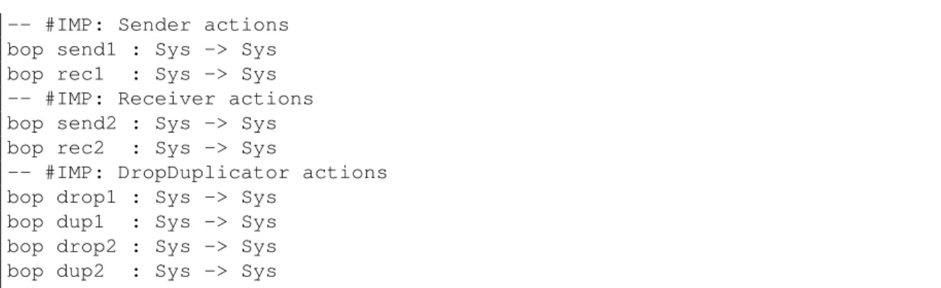
Each transition is performed by only one thread in the Java program and we also need to decide which thread to perform the corresponding transition. Comments are used as directives for programmers to know which threads will execute each transition. The transition’s condition becomes the precondition of the method implementing the transition and by looking at the change of observers in the OTS, we know how to implement the method’s body.

(38)

-- #IMP: Sender actions bop send1 : Sys -> Sys bop rec1 : Sys -> Sys -- #IMP: Receiver actions bop send2 : Sys -> Sys bop rec2 : Sys -> Sys

-- #IMP: DropDuplicator actions bop drop1 : Sys -> Sys

bop dup1 : Sys -> Sys bop drop2 : Sys -> Sys bop dup2 : Sys -> Sys

For example, Listing 5.3 shows transitions of ABP’s specification with their comments. The transitions send1 and rec1 are performed by the sender, send2 and rec2 are performed by the receiver and four transitions drop1, dup1, drop2 and dup2 are be performed by another thread called drop-duplicator.

5.1.3 Step3: Program design in Java

We apply state pattern represented in 4.2.2 to write concurrent programs in this project. There is one minor difference between diagrams in the Figure 5.1 and Figure 4.1 is that now Context is a subclass of Thread in Java so that it can be used to create threads in Java applications. Attributes that are mapped from observers are stored in the context of each thread. One thread has several states represented by separated classes and all concrete states are child classes of a state abstract class.

Figure 5.1: Programe design in Java

The state abstract class has a move method which is implemented differently in concrete child classes. Each transition of the OTS will be implemented in the move methods of each state. On the finish of each transition, the thread changes its state by setting a new state to its context.

(39)

5.2 Case studies

5.2.1 ABP Simulator

From a part of ABP’s specification showed in the Listing 5.1, we have identified that there are three threads in the simulator: sender, receiver and drop-duplicator. Six observers of ABP specification and their distribution to threads are shown in Listing 5.2.

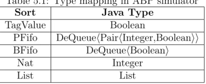
Table 5.1 shows the type mapping of each variable in Java program depending on the sort of observers in the OTS.

Table 5.1: Type mapping in ABP simulator

Sort Java Type

TagValue Boolean

PFifo DeQueuehPairhInteger,Booleanii

BFifo DeQueuehBooleani

Nat Integer

List List

Six transitions in ABP specification and information on which thread performs each transition are shown in Listing 5.3. After mapping observers and transitions, we can visualize the state machines of sender and receiver in Figure 5.2.

Figure 5.2: State machine of the sender and receiver

The drop-duplicator thread can also be implemented as a state machine using the pattern in Section 5.1.3 but the order of transitions it performs is not fixed. It can arbitrarily perform one of the four transitions at any time, then we decide to implement it as a normal thread where the drop and duplication are performed in a while loop and we do not talk about its structure here.

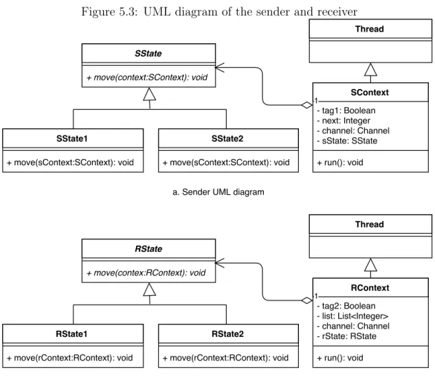
Next, we represent the structure of the sender and the receiver of the simulator. Fig. 5.3 shows the UML diagrams of the sender and receiver. The sender’s context includes attributes tag1 and next that are mapped from observers, a reference to the global channel and a state variable sState. Similarly, the receiver’s includes tag2 and list, a reference to the global channel and a state variable rState. When the sender and receiver start running, they may change their states by setting the new state to its context.

There are two possible states for the sender which are represented by two classes SState1 and SState2 in Java. The move methods of SState1 class will implement the send1

(40)

Figure 5.3: UML diagram of the sender and receiver

transition and the move methods of SState2 class will implement the rec1 transition. Transition rec2 is implemented in the move method of class RState2 and transition send2 is implemented in the move method of class RState2.

A transition is implemented in Java according to its equations in the OTS and we choose rec1 as a demonstration. The semantics of rec1 transition in the OTS is shown in Listing 5.4.

Listing 5.4: Transition rec1 in ABP

op c-rec1 : System -> Bool

eq c-rec1(S) = not empty?(fifo2(S)) . eq fifo1(rec1(S)) = fifo1(S) .

ceq fifo2(rec1(S)) = get(fifo2(S)) if c-rec1(S) .

ceq tag1(rec1(S)) = (if tag1(S) = top(fifo2(S)) then tag1(S) else top( fifo2(S)) fi) if c-rec1(S) .

eq tag2(rec1(S)) = tag2(S) .

ceq next(rec1(S)) = (if tag1(S) = top(fifo2(S)) then next(S) else s(next(S )) fi) if c-rec1(S) .

(41)

eq list(rec1(S)) = list(S) .

-- IMP: change state without modifying observers ceq rec1(S) = S if not c-rec1(S) .

The condition c-rec1 of rec1 transition comes true if fifo2 is not empty. By looking at the changes of observers in the specification, we know that if the condition c-rec1 is satisfied, values of fifo2, tag2, list are not changed, values of tag1 and next are changed based on equality of the current value of tag1 and the top of fifo2. From these information, we implement move method in class SState2 as in Listing 5.5:

Listing 5.5: Java method for rec1 transition public void move(SContext sContext) {

Boolean ack = sContext.getChannel().getAck();

if (ack != null) { if (ack != sContext.getTag1()) { sContext.setTag1(!sContext.getTag1()); sContext.setNext(sContext.getNext() + 1); } }

SState sState = new SState1(); sContext.setsState(sState); }

In the function, the checking ack != null corresponds to c-rev1 condition in the OTS and the checking ack != sContext.getTag1() is used as a condition to change values of tag1 and next in the transition. On the finish of this transition, the context is set to a new state SState1.

The receiver is implemented in the similar way and the main class of the program will initialize the data and start both sender and receiver in the program.

5.2.2 Simple Cloud Simulator

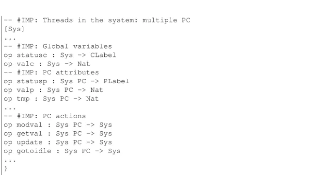
Simple cloud is a protocol used for synchronization of a natural number between one cloud computer and many PCs. We can think of this number as a revision in Git control, so now we call it revision number. The cloud computer can be in two status: IDLE and BUSY, and each PC can be in three status: IDLE, GOTVAL, UPDATED. One PC can only connect to the cloud computer only if it is in IDLE status and the cloud is also IDLE. In this case, the cloud’s status goes into BUSY and the PC’s one goes into GOTVALUE where it obtains revision number from the cloud. After that, the PC compares the revisions, updates them according to the highest value and goes into UPDATED status. From the UPDATED status, the PC goes back into IDLE status and the cloud also goes into IDLE status. A part of simple cloud’s OTS showed in Listing 5.6 lets us know information about threads, variables and actions performed by each thread in the simulator.

Listing 5.6: Simple Cloud specification

(42)

-- #IMP: Threads in the system: multiple PC [Sys]

...

-- #IMP: Global variables op statusc : Sys -> CLabel op valc : Sys -> Nat

-- #IMP: PC attributes

op statusp : Sys PC -> PLabel op valp : Sys PC -> Nat

op tmp : Sys PC -> Nat ...

-- #IMP: PC actions

op modval : Sys PC -> Sys op getval : Sys PC -> Sys op update : Sys PC -> Sys op gotoidle : Sys PC -> Sys ...

}

There will be multiple PC threads running in the simulator and each thread has three attributes representing the status, revision number and a temporary revision got from the cloud computer. The global variables include the status and revision number of the cloud. All four transitions in the specification are performed by PC threads.

Next, let us see the implementation of the simulator in Java. Figure 5.4 and Figure 5.5 illustrate the state and UML diagrams of each PC in the program respectively.

Figure 5.4: State diagram of each PC

There are four possible states for each PC and each PC’s initially state is PState1. The modval transition operator from the specification has two parameters and one of them is the id of one PC whose sort is PC in CafeOBJ. This transition is implemented by the move method in PState1 class. Transitions getval, update and gotoidle are implemented in classes PState2, PState3 and PState4 respectively. A new state is set to the thread context after successfully executing one transition in each move method.

Table 5.2 demonstrates the mapping from sorts of observers to Java types.

Table 5.2: Type mapping in Simple Cloud

Sort Java Type

CLabel enum CStatus PLabel enum PStatus

(43)

Figure 5.5: UML diagram of each PC

Now, we look at the implementation of transitions in Java code. We choose the transi-tion update as an example. The definitransi-tion of update in the OTS is showed in Listing. 5.7 and the move method in Java for this transition is in Listing. 5.8.

Because this method accesses and modifies global data, there must be a synchronization on global data between threads. The condition of update transition says that this transi-tion is enabled only if the cloud’s status is BUSY and the thread’s status is GOTVALUE. This condition is translated into the checking condition of the move method of PState3. The changes of observers in the OTS are translated to the method’s body in Java. On the finish of this method, a new state of type PState4 is set to the PC context. In the similar way, other transitions can be implemented in corresponding states.

Listing 5.7: update transition in Simple Cloud OTS

mod* CLOUD { ...

op c-update : Sys PC -> Bool

eq c-update(S,I) = (statusc(S) = busy and statusp(S,I) = gotval) . eq statusc(update(S,I)) = statusc(S) .

ceq valc(update(S,I)) = (if tmp(S,I) <= valp(S,I) then valp(S,I) else valc(S) fi) if c-update(S,I) .

ceq statusp(update(S,I),J)= (if I = J then

updated else statusp(S,J) fi) if c-update(S,I) . ceq valp(update(S,I),J) = (if I = J then

(if tmp(S,I) <= valp(S,I) then valp(S,I) else tmp(S,I) fi) else valp(S,J) fi) if c-update(S,I) .

ceq tmp(update(S,I),J) = (if I = J then

(if tmp(S,I) <= valp(S,I) then valp(S,I) else tmp(S,I) fi) else tmp(S,J) fi) if c-update(S,I) .

ceq update(S,I) = S if not(c-update(S,I)) . ...

(44)

}

Listing 5.8: Java method for update transition in PState3 public void move(PContext pContext) {

synchronized (pContext.getCloud()) {

if (pContext.getStatus() == PStatus.GOTVAL && pContext.getCloud(). getStatus() == CStatus.BUSY) { if (pContext.getTmp() <= pContext.getVal()) { pContext.getCloud().setVal(pContext.getVal()); pContext.setTmp(pContext.getVal()); } else { pContext.setVal(pContext.getTmp()); } pContext.setStatus(PStatus.UPDATED); PState pState4 = new PState4(); pContext.setpState(pState4); }

} }

5.2.3 Qlock Simulator

Qlock is another case study we want to represent in this report. This is a well-known mutual exclusion protocol [8] in which many agents are trying to access a global resource and only one can be allowed at a time. In order to do that, the protocol use a queue to control the agents’ access. Once an agent wants to use the global resource, it has to put its id to the queue first and waits until its id is on top of the queue. After releasing the resourse, its id is removed from the queue. Listing 5.9 shows observers and transitions in the OTS specification of Qlock.

Listing 5.9: Qlock specification

mod* QLOCK {

-- #IMP: Threads in the system: multiple Agents [Sys]

...

-- #IMP: Global variables op queue : Sys -> Queue -- #IMP: Agent attributes op pc : Sys Pid -> Label ...

-- #IMP: Agent actions bop want : Sys Pid -> Sys bop try : Sys Pid -> Sys bop exit : Sys Pid -> Sys ...

(45)

Observer queue is used to observe the value of global queue. Program counter of an agent is kept track by the pc observer and it has three possible values l1, l2 or cs which are elements of Label sort. Initial label of an agent is l1 and it will be updated to l2 if the agent successfully puts its id to the queue by want transition. When an agent accesses the global resource by performing try transition, its pc value will be cs and the pc comes back to l1 when it releases the resource by performing exit transition.

From the annotations in the OTS, programmers are supposed to write a concurrent program including many Agent threads. The state and UML diagram of each agent are illustrated in Figure 5.6 and Figure 5.7.

Figure 5.6: State diagram of each agent

Figure 5.7: UML diagram of each agent

Each thread has pc and aid attributes to keep track of its program counter and id respectively. The Label sort is mapped to an enum type which has three values in Java and Integer is used for Pid sort. All the transitions in the OTS are performed by each agent.

Now let us see the implementation of one transition in Java and we choose try transition for the demonstration. The specification of try transition is showed in Listing 5.10 and its implementation is described in Listing 5.11.

Listing 5.10: try transition of Qlock

op c-try : Sys Pid -> Bool

eq c-try(S,I) = (pc(S,I) = l2 and top(queue(S)) = I) .

(46)

eq queue(try(S,I)) = queue(S) . ceq try(S,I) = S if not c-try(S,I) .

Listing 5.11: Java method for try transition in AState2 public void move(AContext aContext) {

if (aContext.getPc() == Label.L2 && aContext.getQueue().getFirst() == aContext.getaId()) {

aContext.setPc(Label.CS);

AState aState3 = new AState3(); aContext.setaState(aState3); }

}

The condition of try transition in the OTS specification is translated into the condition of if statement in Java. If it is satisfied, the agent’s state is changed to AState3 by creating a new state object of this type and assigning it to the agent’s context.

In addition, the same techniques are also successfully applied to implement NSLPK, an authentication protocol mentioned in [15, 16] to exchange keys between agents over an insecure network based on their annotated OTS specifications in CafeOBJ.

5.3 Testing a Java Concurrent Program based on its

OTS Specification

One important issue is to check if an implementation in Java is correct and conforms to its OTS specification in CafeOBJ or not. In this section, we represent two approaches that has been applied to our projects.

5.3.1 Model Check the Implemenation with JPF

The first approach simply uses JPF to model check our concurrent Java programs. Prop-erties required for the systems are expressed by assertions in Java. One advantage of this approach is that we can exhaustively traverse the whole state space of a Java program but for a pretty big program, it is impossible to be checked by JPF. Here we report some cases that can be model checked in JPF.

• Testing result for ABP simulator: In order to check if the receiver gets correct result from the sender, we add an assertion based on the next value on the sender and the list on the receiver after they finish. If we initiate one drop-duplicator in the simulator, the system’s state space increases significantly, therefore the following results are reported for the simulator without any drop-duplicator.

Listing 5.12: JPF result from ABP simulator (data channel size = acknowledge channel size = 1, number of packages = 1)

JAIST Repository: Program development in Java based on CafeOBJ specifications [課題研究報告書]