JAIST Repository: Agent-Based Modeling on Technological Innovation as an Evolutionary Process

JAIST Repository

https://dspace.jaist.ac.jp/

Title

Agent-Based Modeling on Technological Innovation

as an Evolutionary Process

Author(s)

Ma, Tieju; Nakamori, Yoshiteru

Citation

European Journal of Operational Research, 166(3):

741-755

Issue Date

2005-11-01

Type

Journal Article

Text version

author

URL

http://hdl.handle.net/10119/5027

Rights

NOTICE: This is the author's version of a work

accepted for publication by Elsevier. Tieju Ma

and Yoshiteru Nakamori, European Journal of

Operational Research, 166(3), 2005, 741-755,

http://dx.doi.org/10.1016/j.ejor.2004.01.055

Description

Tieju Ma and Yoshiteru Nakamori, Agent-Based Modeling on Technological

Innovation as an Evolutionary Process, European Journal of Operation Research,

Elsevier Science, 2004. (In press)

Agent-based modeling on technological innovation as an

evolutionary process

Tieju Ma and Yoshiteru Nakamori

∗

School of Knowledge Science

Japan Advanced Institute of Science and Technology

1-1, Asahidai, Tatsunokuchi, Ishikawa 923-1292, Japan

February 20, 2004

Abstract

This paper describes a multi-agent model built to simulate the process of technological innovation, based on the widely accepted theory that technological innovation can be seen as an evolutionary process. The actors in the simulation include producers and a large number of consumers. Every producer will produce several types of products at each step. Each product is composed of several design parameters and several performance parameters (fitness components). Kauffman’s famous NK model is used to deal with the mapping from design parameter space (DPS) to performance parameter space (PPS). In addition to the constructional selection, which can be illustrated by the NK model, we added environmental selection into the simulation and explored technological innovation as the result of the interaction between these two kinds of selection.

Keywords: agent-based simulation; technological innovation

1

Introduction

In recent years, agent-based modeling (ABM) has become increasingly influential in many fields of social science such as economic, political, anthro-pological, and so on. The examples of such works include [17, 4, 7, 11, 22, 6]. It is widely believed that ABM is not only a new powerful tool for re-searchers to challenge complex adaptive systems [16], but also a new way of thinking about the world where we live. The main purpose of ABM is to study the macro-level complexities from the interactions in the micro-level, in other words, ABM tries to challenge complexities in a bottom-up way. Researchers doing ABM, especially in so-cial simulations, always keep in mind that “simple patterns of repeated individual action can lead to extremely complex social institutions” [8].

Agents in the ABM can be simply defined as autonomous decision-making entities. From a more theoretical view of artificial intelligence, an agent is a computer system that is either concep-tualized or implemented using the concepts that are more usually applied to humans [24]. Simply speaking the purpose of this research is to model and simulate the technological innovation process by ABM.

There are good reasons to view innovation systems as complex systems. The actors of the system interact with each other, learn, adapt and reorganize, expand their diversity, and explore their various options [20]. And one of the ob-vious features of technological innovation in an advanced industrial society is that it involves the coevolution of marketable artifacts, scientific con-cepts, research practices and commercial orga-nization [25]. Many researchers suggested that technological innovation should be understood as an evolutionary process [9, 13, 19, 25]. Techno-logical innovation is also featured as a complexity challenge [2].

Based on the above thinking, many different models about technological innovation have been developed. Roughly, those models can be divided into two groups. The first group focuses on in-dustrial firms, treating them as social organiza-tions driven by market forces to adapt to

chang-ing technological regimes. Such models abound in literatures of evolutionary economics [23]. The second group focuses on the essence of technolo-gies themselves. Typical models in this group are Arthur’s [5] model of the “lock-in” of a sin-gle, but potentially sub-optional technology and Kauffman’s [12] NK model of hill-climbing which predicts potentially different sub-optima in a rugg-ed fitness landscape. The first group tries to cap-ture the feacap-tures of technological innovation from macro level, while the second group tries to ex-plain technological innovation from micro level. Considering technologies (or its carrier products and services) as species, the first group pays much attention to the environment in which the species live, while the second group pays much attention to how the physical structure of individuals, for example DNA, affects the behavior and future of the species.

This paper presents an agent-based model that integrates the basic ideas of both groups. In our model, there are mainly two kinds of actors (or agents), producers and consumers. Producers de-sign and produce different products. Consumers evaluate and purchase those products. As the car-rier of technologies, every product is composed of several design parameters. And as commodities, products have performance parameters which can bring utilities to consumers. The mapping from design parameter space (DPS) to performance pa-rameter space (PPS) is dealt with by using Kauff-man’s NK model. The agent-based model indi-cates our basic conceptual understanding about technological innovation: an innovation in tech-nology is the result of both constructional selec-tion and environmental selecselec-tion.

Constructional selection can be seen as a kind of inner selection. In the process of technological innovation, there is some outside pull or pressure, that is to say, the social environment, especially market forces, will play an important role in se-lection. Corresponding to constructional selec-tion, the impact from the environment is called environmental selection. Constructional selection generates things with high performance, but it doesn’t mean these things will be overwhelming in environmental selection. The survivors are the

result of both types of selection.

Based on the agent-based model, we devel-oped a platform by using object-oriented program-ming to simulate the technological innovation pro-cess under different situations. The methodology we have adopted accords with Axelrod’s descrip-tion of the value of simuladescrip-tion [9]:

Simulation is a third way of doing sci-ence. Like deduction, it starts with a set of explicit assumptions. But un-like deduction, it does not prove theo-rems. Instead a simulation generates data that can be analyzed inductively. Unlike typical induction, however, the simulated data comes from a rigorously specified set of rules rather than direct measurement of the real world. While induction can be used to find patterns in data, and deduction can be used to find consequences of assumptions, sim-ulation modeling can be used to aid in-tuition [3].

2

The agent-based model

2.1

Producers, consumers, and

map-ping from DPS to PPS

Two kinds of actors are included in the model, producers and consumers. Here the producers belong to the same industry, for example the au-tomobile industry. The set of producers can be denoted as:

P=_{P1,· · · , PS}. (1)

The set of consumers can be denoted as:

C=_{C1,· · · , CR}. (2)

In every time step, producer Pi(i = 1,· · · , S) will

produce Li types of products.

AP i={Ai1,· · · , AiLi}, i = 1, · · · , S. (3)

As the carrier of technologies, every product is composed of N design parameters, and as a

commodity, every product has U performance pa-rameters which can bring utilities to consumers. For consumers, design parameters hide behind performance parameters. For example, when pur-chasing a digital camera, consumers will consider “compatibility” which can be considered a perfor-mance parameter. Most consumers will not con-sider whether the camera uses a serial or parallel interface because they don’t understand what a serial or parallel interface is. But for the tech-nicians who design digital cameras, “interface” is a design parameter they must consider, and “se-rial” and “parallel” are two design values of this design parameter. The “interface”, with other design parameters, will decide the “compatibil-ity” of a digital camera. Also the “interface” will influence other performance parameters, such as the “appearance” of a digital camera. From the above example, we can see that the relationship between design parameters and performance pa-rameters is something like a genotype-phenotype map.

The NK model is used to illustrate the map-ping from DPS to PPS because it explicitly shows the epistatic structure of the genotype-phenotype map. In the NK model, N represents the number of genes in a haploid chromosome and K repre-sents the number of linkages that each gene has to other genes in the same chromosome [13]. Re-garding the design parameters as genes, following L. Altenberg [1], the traditional NK model can be described as the following:

• The genome consists of N genes (design pa-rameters) that exert control over U phe-notypic performance parameters, each of which contributes a component to the total fitness (performance).

• Each gene controls a subset of the U perfor-mance parameters, and in turn, each per-formance parameter is controlled by a sub-set of the N genes. This genotype-phenotype map can be represented by a matrix, M= (mij)_N×U, i = 1,· · · , N ; j = 1, · · · , U,

(4) of indices mij ∈ {0, 1}, where mij = 1

pa-rameter j. M is randomly initialized in the simulation. M will be static unless the DPS or PPS changes.

• The columns of M, called the polygeny vec-tors, qj = (mij)N×1(i = 1, . . . , N ), give

the genes controlling each performance pa-rameter j.

• The rows of M, called the pleiotropy vec-tors, qi= (mij)1×U(j = 1, . . . , U ), give the

performance parameters controlled by each gene i.

• If any of the genes controlling a given per-formance parameter mutates, the new value of the performance parameter will be un-correlated with the old. Each performance parameter is a uniform pseudo-random func-tion of the genotype, x_{∈ {0, 1}}N

fi= f (x◦ qi; i, qi)∼ uniformon[0, 1]. (5)

Where

f :_{{0, 1}}N_{× {1, · · · , N } × {0, 1}}N _{→ [0, 1].} (6) Here_{◦ is the Schur product.}

x_{◦ q}i = (ximij)_N×1(i = 1, . . . , N ).

Any change in i, qi, or x◦ qi gives a new

value for f (x_{◦ q}i; i, qi) that is uncorrelated

with the old.

• If a performance parameter is affected by no genes, it is assumed to be zero.

fi= 0, if qi= (0· · · 0) . (7)

• Total fitness is defined as the normalized sum of the performance parameters:

F C = 1 U U X i=1 fi. (8)

We make one change to the traditional NK model: the genes are not binary-valued, but Hi

-valued, i.e., in our model, the gene i has Hivalues,

not just the two values 0 and 1. This is accept-able because it is not necessary that every design

parameter has only two design values. For exam-ple, considering “engine” as a design parameter when designing a new car, technicians can select from dozens of different engines.

Thus the x _{∈ {0, 1}}N in Eq. (5) and Eq. (7) should be changed into x_{∈ {1, · · · , H}i}N(i =

1,_{· · · , N ), and the Eq. (6) should be modified to} be:

f :_{{1, · · · , H}i}N × {1, · · · , N} × {1, · · · , Hi}N

→ [0, 1](i = 1, · · · , N ).

We can suppose there is a general DPS [21] G which includes all the design values of the N design parameters.

G= (g1,· · · , gN)T. (9)

Here T means transpose.

For every design parameter gi(i = 1,· · · , N )

in G, it has Hi values.

gi= (gi1,· · · , giHi), i = 1,· · · , Hi. (10)

For every producer, the values of its design parameters are generated from the G, i.e.

GP i⊆ G, i = 1, · · · , S. (11)

For example, if N = 4 and Hi = 3(i = 1,· · · , 4),

the G and the DPS of a certain producer Pi∗are:

G=     g11 g12 g13 g21 g22 g23 g31 g32 g33 g41 g42 g43     and GP i∗=     g11 0 g13 g21 0 0 g31 0 g33 0 g42 g43     .

In Gpi∗ the 0 means producer Pi∗ has no such

design value corresponding to the position in G. Any product is composed of N design parameters. Now we can calculate that with Gpi∗the producer

Pi∗ can produce 8 types of products: A_{P i∗}=                        A_i∗1=_{g11, g21, g31, g42} A_i∗2=_{g11, g21, g31, g43} A_i∗3=_{g11, g21, g33, g42} A_i∗4=_{g11, g21, g33, g43} A_i∗5=_{g13, g21, g31, g42} A_i∗6=_{g13, g21, g31, g43} A_i∗7=_{g13, g21, g33, g42} A_i∗8=_{g13, g21, g33, g43}                        .

The U performance parameters of products can be denoted as:

F=_{f1,· · · , fU}. (12)

2.2

Purchasing behavior

A consumer’s purchasing behavior can be sim-ply described as: he/she evaluates several types of products, and select one whose utility is the biggest for him/her among those types evaluated by him/her. Now the problem is to model how consumers evaluate products. We consider the following three different evaluation methods. Each method is based on different philosophy, but a dis-cussion of these philosophies is beyond the scope of this paper.

2.2.1

Weighted average method

In this method, for any consumer Cj (j = 1,

. . . R), its weights for different performance pa-rameters can be denoted as:

WCj ={w1Cj,· · · , wU Cj}, j = 1, · · · , R. (13) subject to ½ wiCj∈ [0, 1], i = 1, · · · , U PU i=1wiCj = 1. (14) A consumer’s evaluation for a type of product is:

E =

U

X

i=1

wifi (15)

Every consumer will select the product which has the biggest E for him/her among those products evaluated by him/her.

2.2.2

Ideal point method

In this method, every consumer has an ideal prod-uct in his/her mind. Eq. (16) gives the distance between design performance of products as they are evaluated by a consumer:

D =

U

X

i=1

(fi− fi0)2 (16)

In Eq. (16), fiis the value of the ith performance

parameter of the products evaluated by the con-sumer, and f0

i is the value of the ith performance

parameter of the consumer’s ideal product. Ev-ery consumer will select the product which has the smallest D for him/her among those products evaluated by him/her.

2.2.3

Max-min method

Supposing, before selecting a product, a consumer will evaluate I types of products which can be de-noted as: Performance Parameter1 · · · Performance ParameterU Product1 f11 · · · f1u .. . ... . .. ... ProductI fI1 · · · fIU

Here fij(i = 1,· · · , I)(j = 1, · · · , U ) is the value

of ith product’s jth performance parameter. If fi∗_j= max

i {min {fij}}, i = 1, · · · , I; j = 1, · · · , U.

(17) Then product i∗will be selected by the consumer. Of course, there are many other evaluation methods. Our model and the platform have an open structure, i.e., researchers can define their own evaluation methods, parameters and even agents’ behavior to do simulation under different assumptions and conditions.

2.3

Constructional selection and

en-vironmental selection

Loet Leydesdorff executed simulation on the com-plex dynamics of technological innovation by

us-ing cellular automata [14]. He explored the in-novation process and results from the viewpoint of constructional selection. In our research, we would like to simulate the innovation process by considering the interaction between constructional selection and environmental selection.

Constructional selection means the selection is based on construction and epistatic performance of the product; it does not consider the situation or environment in which the product exists. En-vironmental selection, on the other hand, means “selected by environment”. Here the environment is something like social environment. It refers to consumers, government regulations, and so on. But for the sake of simplicity, we just consider consumers in this paper.

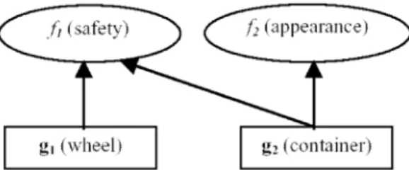
Here we present an example to illuminate structional and environmental selection by con-sidering a kind of simple vehicle. Supposing there are two design parameters, wheel and container, for designing a vehicle, every design parameter has two design values, as shown in Fig. 1.

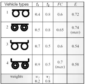
Two performance parameters of the vehicles are considered, safety and appearance. Fig. 2 shows a genotype-phenotype map which indicates that the safety is affected by both wheel and con-tainer, but the appearance is affected only by the container.

Figure 1: The DPS of a kind of vehicle.

According to the DPS, four types of products can be produced, as shown in the first column of Table 1. The values of f1 and f2 (the second

and third columns of Table 1) are obtained ac-cording to Eq. (5). Then the values of FC in the fourth column can be obtained according to Eq. (8), and the type 4 will be selected by construc-tional selection which is based on FC. If, however,

Figure 2: The genotype-phenotype map.

consumers’ weight for safety is 0.2 and weight for appearance is 0.8, then according to Eq. (15), the values in the fifth column of Table 1 can be obtained, and type 2 will be selected by environ-mental selection which is based on E.

2.4

Product evolution

In this paper, the environment mainly refers to market, so environmental selection is also called market selection. In fact, the market selection is very complex, related to each consumers’ prefer-ences, cultural background, income, age, sex, and so on. For the sake of simplicity, we assume a sim-ple purchasing model: in every time step, every consumer will evaluate a certain number of prod-uct types, and purchase the one that he/she rates the highest. In order to survive, producers must continue to design new products which will bet-ter meet consumers’ preferences. The products which can have higher utility will be more likely to retain their characteristics in the next gener-ation of products. We use the following genetic algorithm [10] to simulate product evolution.

The set of all product types in the market at a certain time step can be supposed as:

A=_{A1,_{· · · , AB}.} (18) For every product type Au (u =1, . . . , B) in A,

if its sale volume is su, then we can get the sale

volume set for every type:

S=_{s1,_{· · · , sB}.} (19) Supposing sminis the minimal value in set S,

Table 1: Constructional selection and

envi-ronmental selection

set A, its probability of being the genome type of the next generation products is:

P (Au) = (su− smin)/ B

X

j=1

(sj− smin). (20)

The new products are generated from genome types by crossover and mutation. The crossover process can be described as: for two selected geno-me types, their chromosogeno-me strings are cut at some randomly-chosen position, thus two “head” segments and two “tail” segments are produced, and the tail segments are then swapped over to form two new full-length chromosomes (product types). It is not necessary that crossover be ap-plied to all pairs of genome types selected for gen-erating new types. Users can specify a probabil-ity for crossover, which is called crossover rate. In this paper, the crossover rate is:

α_{∈ (0, 1).} (21)

Crossover makes offspring inherit some genes from each parent, while mutation will enable off-spring to have genes that their parents do not

have. Each gene (design parameter) of offspring will mutate according to a probability called mu-tation rate, which is also specified by users. In this paper, the mutation rate is:

β _{∈ (0, 1).} (22)

As shown in Eq. (10), for design parameter gi(i = 1,· · · , N), it has Hi design values. If a

mutation happens to gi(i = 1,· · · , N), each

de-sign value will have the same probability, which is 1/Hi, to be selected as the value of this design

parameter.

3

Simulation

Based on the model introduced above, we built a platform. On this platform, not only can we set different values for all the parameters men-tioned above, but also define different behaviors of the agents. Similar to Nigel Gilbert’s state-ment [9], the role of simulation in this paper is not to create a facsimile of any particular inno-vation that could be used for prediction, but to use simulation to assist in the exploration of the consequences of various assumptions and initial conditions. In the following we will execute simu-lations under different situations and discuss the results of those simulations.

Three evaluation methods—weighted average, ideal point and max-min— were mentioned in Sec-tion 2.2. Although the following simulaSec-tions main-ly focus on the weighted average method, simu-lations on the other two evaluation methods are also simply introduced.

The basic initializations for all the following simulations are:

• N = 6, U = 5, and Hi = 4 (i = 1, . . . , 6),

which means every product is composed of 6 design parameters and has 5 perfor-mance parameters, and every design pa-rameter has 4 design values. So in total there can be 64 _{= 1296 types in the}

indus-try. The mapping from DPS to PPS , the M in Eq. (4), is randomly initialized.

• S = 3, Li= 50(i = 1, . . . , 3), which means

there are three producers, and at each time step, every producer will produce 50 prod-uct types. Each producer’s initial types are randomly generated from their DPS. • R = 1000, which means that altogether

there are 1000 consumers.

• α = 0.7, β = 0.02, which means the crossover rate is set to 0.7 and the mutation rate is set to 0.02.

The genotype-phenotype map from DPS to PPS is initialized randomly, and in most of the situations, the products evaluated by consumers are randomly selected from the market. Thus the result will be different almost every time we run the program. The absolute values in the output make no sense. What makes sense is the pattern of the output based on the time step. We ran simulations 30 times for each situation. The re-sults shown in the following are typical patterns in different situations.

3.1

Based on weighted average

me-thod

We assume that all consumers evaluate products by using the weighted average method. In the simulation, we consider two measures. One is the average evaluation value (AVE) of all consumers for all product types, which can be denoted as:

AV E = R P i=1 S P j=1 Lj P l=1 Eijl R_× S P j=1 Lj (23)

Here, Eijl means the evaluation value of

con-sumer Ci to the product type Ajl produced by

producer Pj. AVE can be used to indicate how

consumers are satisfied with the industry. The other is the average performance value (AVF) of all products, which can be denoted as:

AV F = S P i=1 Li P j F Cij S P i=1 Li (24)

Here the FCij means the constructional fitness

of type Aij produced by producer Pi, and it is

obtained according to Eq. (8). AVF can be used to indicate the maturity of an industry. In the following, we will consider several situations.

3.1.1

Situation 1

In this situation, we assume:

• All consumers’ weight sets are the same, which means all consumers have the same weight for the same performance parame-ter.

• All consumers are fully informed about the market, which means when one consumer wants to buy a product, he/she will evalu-ate all product types available in the mar-ket place and select the one which he/she rates the highest.

• The three producers’ DPS are randomly generated from the general DPS (the DPS of the whole industry), and will not change during the simulation.

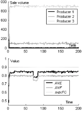
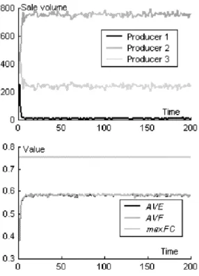
The top part of Fig. 3 shows the sale records (sale volume at each time step) of the three pro-ducers. We can see producer 3 monopolizes the market, and producer 1 and producer 2 can sale nothing. This is not to say that producer 3 will always be the monopolist. In almost every sim-ulation, a monopoly appears, and the three pro-ducers have an equal chance to be the monopolist. Because all the consumers have the same weight for the same performance parameter, the market will select types which have the maximal E for all consumers. According to the Eq. (8), mostly there is only one type with maximal E, but it is possible that more than two types have the same maximal E by accident. And according to the NK model, or Eq. (4), (5), (6), (7) and (8), it is also possible that accidentally more than two producers produce product types with maximal E for all consumers.

The lower part of Fig. 3 shows the AVE, AVF and maxFC, where maxFC is the maximal FC of all possible product types. We can see AVE

Figure 3: The result of situation 1.

and AVF frequently show large changes. Those changes are caused by the mutation of products. Because the whole market are overwhelmed by one type (or several types with small possibil-ity as discussed above), the mutation of this type will affect all consumers’ E, and because all con-sumers have the same weight for the same per-formance parameter, the affection is identical for all consumers, that means the affection for dif-ferent consumers can’t be neutralized when cal-culating AVE. The mutation of the overwhelm-ing type will cause changes to F C of all prod-ucts in the market place, and those changes also can not be neutralized when calculating AV F . In Fig. 3, the changes of AVE and AVF are not completely synchronous. This is reasonable if we analyze the Eq. (8) and the Eq. (15) more — an increase/decrease in FC does not have to result in an increase/decrease in E. From the view of the market, an improvement of products

does not have to result in a business success un-less the improvement is what consumers really need and consumers attach importance to the im-provement. What we can learn from the simula-tion and analysis is: it is very important to in-tegrate both the technological knowledge (knowl-edge about technology) and consumer knowl(knowl-edge (knowledge about consumer) into the new prod-ucts for getting business success [15].

3.1.2

Situation 2

The assumptions in this situation are the same as those in situation 1 except that consumers are only partly informed about the market, which means when a consumer shops, he/she will eval-uate some (5 types), not all, of the products, and those types are randomly selected from all the types available in the market place.

Figure 4: The result of situation 2.

As shown in Fig. 4, although producer 1

oc-cupies most of the market, it can not completely monopolize it. Other producers can sell some-thing, and comparing with the result in situation 1, there is almost no big change to AVE and AVF except at the beginning of the simulation. There are drops in AVE and AVF at about time step 80. The drops were caused by a mutation in products. This mutation decreased both AVE and AVF, in other words, this mutation did harm to the pre-vious technical structure. But we can see produc-ers finally overcame the harm. Such phenomenon can be explained as: technicians apply a new de-sign value without knowing this dede-sign value is not good for the current technical structure un-til the products come into the market. In the real world, a good producer can overcome such bad mutations during the period of test before forwarding the products to the market.

3.1.3

Situation 3

Figure 5: The result of situation 3.

In this situation we assume:

• There are 50 consumer weight sets, which means there are 50 kinds of consumers. • Consumers are partly informed about the

market.

• The three producers’ design spaces are ran-domly generated from the general design space, and will not change during the sim-ulation.

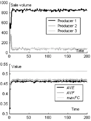
In this situation we find that although one producer (producer 1 in Fig. 5) can occupy most of the market in most of cases, it can not com-pletely monopolize the market, and other pro-ducers can have some (small) market share. In Fig. 5, AVE and AVF are more stable than be-fore. This is because the diversity of consumers’ demand leads to the diversity of products, thus those changes to FC for individual product and E for individual consumer can counteract each other.

3.1.4

Situation 4

The assumptions in this situation are the same as those in situation 3 except that almost every consumer’s weight set is different. That means the diversity of consumers’ demand is higher than that in situation 3.

As shown in Fig. 6, there is no monopoly in the market. Because of the high diversity of con-sumers’ demand, it is very difficult for any single producer’s products to satisfy all consumers. One thing we have not expected is that AVE almost equals AVF in this situation, which really leads us to think more about the underlying mecha-nisms. We realize that, in this situation, any sin-gle consumer’s preference can not dominate the direction of product improvement, and the im-provement of products is mainly dominated by products’ performance parameters. For a prod-uct in the market place, the deviation of different consumers’ evaluation will counteract each other, and the final effect is that AVE approximates to AVF.

Figure 6: The result of situation 4.

By comparing the results in the above four situations, we find two factors that could pro-tect the market being completely monopolized by producers who make better technological innova-tion than others. The first factor is consumers’ incomplete information. In the first situation, producer 3 (in Fig. 3) occupied all the market because it made better innovation in its prod-ucts and all consumers realized this innovation; while in the rest three situations, it was possi-ble that a producer made great innovation, but not all of consumers realized it because they were partly informed about the market. The second factor is the diversity of consumers’ demand. In the first situation, all consumers’ preferences were the same, and there was an apparent monopoly in the market; while in the third situation, the monopoly became weak; and in the fourth situa-tion, we could say there was no apparent monopoly in the market.

A common point in each situation is that AVF is smaller than maxFC that can be looked as the global optimal technological solution in an indus-try, which means it is most likely that an in-dustry is operated under local optimal techno-logical solutions, not the global optimal solution. We believe two factors contributing to this phe-nomenon. One is, there are too many peaks in the rugged landscape of PPS, and it is difficult for an industry to find the highest peak. In the above situations, we ran the simulation for 200 time steps. With more time steps, theoretically, pro-ducers could find the highest peak. So we could not say it is impossible for an industry to find the global optimal technological solution. But it is really difficult for an industry to find the optimal solution, not only because of the large amount numbers of peaks, but also due to the dynam-ics of DPS. The other is, technological innovation is the result of both constructional selection and environmental selection. It is not necessary that the global optimal solution (the highest peak) in constructional selection is also global optimal in environmental selection. Table 1 showed a good example of this factor. The type 4 in Table 1 is a global optimal technical solution in terms of con-structional selection, but consumers are more like type 2.

3.1.5

Situation 5

The general DPS of the whole industry and the DPS of every producer are dynamic. The dy-namics of DPS refers to the expansion of spaces through the addition of new operants and their progressive structuring and articulation [21]. In the real world, the dynamics of DPS are very com-plex. It makes no sense to study the dynamics of DPS of a certain industry without consider-ing that industry’s history and the cultural back-ground. Our aim is not to simulate any real dy-namics of DPS, but to reveals the fundamental dynamics of DPS. For our model, the dynamics of DPS has two forms, the change of design val-ues, and the change of design parameters.

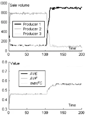
The assumptions in this situation are based on situation 4, in addition, producer 1 will expand

its DPS by finding new design values at time step 100. As introduced above, every producer’s DPS is randomly generated from the general DPS of the industry, in other words, any individual pro-ducers’ DPS does not contain all design values in the general DPS. In this situation, we let pro-ducer 1 get all the design values of the general DPS at time step 100.

Figure 7: The result of situation 5.

As shown in Fig. 7, after expanding its DPS at time step 100, producer 1 moves from being a poor producer to an excellent one. Its mar-ket share increases. And the AVE and AVF also increase after producer 1 expands its DPS, which means consumers have become more satisfied with the industry and the industry is more mature. The reason why producer 1 can become a success-ful one is that its expanded DPS provides more deign values for the genetic algorithm introduced in Section 2.4 to find better technical solutions, and the better technical solutions lead to the in-crease of AVE and AVF.

In the real world, finding new design values is the main way for producers to reinforce their competitive advantages. Theoretically, not every new design value will benefit the producer. New products are always the result of conscious de-sign. Most of the time, those design values which will not benefit the producer will be filtered out during the research and development process.

3.1.6

Situation 6

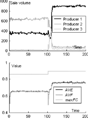
Adding new design parameters into DPS will cause big changes in the technical structure of the prod-uct. The assumptions in situation 6 are based on situation 4, in addition, a new design parameter is added to the industry at time step 100. When

Figure 8: Pattern 1 under situation 6.

we look at AVE and AVF, we see that three pat-terns appear under this situation, and we did not find that any pattern appeared more frequently than another two in the simulation. In pattern 1, both the AVE and AVF increase after adding the

new design parameter, as shown in Fig. 8. That means consumers are more satisfied with the in-dustry and the maturity of the inin-dustry becomes higher.

In pattern 2, shown in Fig. 9, the AVE and AVF first decrease sharply, then climb to a level higher than before the new design parameter was added. In other words, when the new design pa-rameter was first added to the industry, the pro-ducers knew little about how to integrate it with existing design parameter. It took a little time for the producers to benefit from the new design parameter.

Figure 9: Pattern 2 under situation 6.

In pattern 3 (Fig. 10), AVE and AVF first de-crease sharply, then climb to a level lower than be-fore the new design parameter was added. This is because the new design parameter brought more disadvantages than advantages to the current tech-nical structure, or because the industry some-times had difficulty in incorporating the new

de-Figure 10: Pattern 3 under situation 6.

sign parameter. In each of these three patterns, there were quakes in the market, as producers changed their position and then after a period of time, became stable again.

Generally, adding a new design parameter to an industry will lead to changes in the industry and changes of producers’ standing in the mar-ket. It is most likely that the maxFC will in-crease. But that does not mean AVF and AVE will also increase, although most of the time they will. That is to say, adding a new design parame-ter will give the industry a chance to increase the AVF and AVE, but it is possible that the indus-try will miss this chance and make things worse as in pattern 3.

Mathematically, adding a new design param-eter means adding a row to the matrix M in Eq. (4). In our simulation, the values of this new row are randomly initialized and will not change in the simulation. According to Eq. (5), those per-formance parameters affected by the new design

parameter will get new values which have no re-lationship with their old values. This is the main reason for the variety of the result in this situa-tion. We also put forward the model in which the new values are related to the old values [15].

3.2

Monopoly Degree

The word “monopoly” has been used in describ-ing the results in from situation 1 to situation 4. Now, we define monopoly degree as:

µ = maxs Sall

(25) Here µ is the monopoly degree, maxsis the

max-imal sale volume of all the producers at the cur-rent time step, and Sallis the number of all sold

products at the current time step.

We ran the program 10 times for every situ-ation in Table 2, and calculated the average µ at time step 200.

It is also possible to examine the behavior with regard to a time series. But it will result in many lines in a three-dimension space. The randomness, mainly caused by the mutation and crossover of the GA and the consumers’ behavior of selecting products for evaluation before shop-ping, makes those lines rugged. Thus it is not easy to compare the results with regards to a time series. And our purpose is to compare re-sults when market is in relative stable states un-der different situations, rather than how produc-ers reach those stable states. We found time step 200 is a suitable point for this purpose. We ran simulation under each situation 10 times for re-ducing the effect of the above randomness.

The results in Table 2 give us the sense that when the consumers are more homogeneous, and the consumers are better informed about the mar-ket, there is more possibility that a monopoly will appear in the market place by means of techno-logical innovation. We can see, in the third and fourth columns of Table 2, for the weighted aver-age method and the ideal point method respec-tively, the µ increases when consumers become more homogeneous. And when the variety of con-sumers’ demand is the same (in the same row

Table 2: Monopoly degree under different

sit-uation at time step 200

in Table 2), the µ in the market with fully in-formed consumers is higher than that in the mar-ket with partly informed consumers. Table 2 also shows that the weighted averaged method can re-sult in higher degree of monopoly than the ideal point method. Other evaluation methods also can be simulated and compared based on the agent-based model introduced in this paper.

4

Conclusions

In this paper, an agent-based model of technologi-cal innovation as an evolutionary process has been presented. This agent-based model describes tech-nological innovation as a process of both con-structional selection and environmental selection. Several situations were considered and the results of the simulations have been discussed. Through the simulations, this paper identified two factors,

consumers’ incomplete information and diversity of consumers’ demand, which could prevent pro-ducers from monopolizing the market by means of technological innovation. In addition, this pa-per not only intuitively showed that an industry is most likely operated under suboptimal techno-logical solutions, but also suggested two reasons for this issue. The first reason is that there are two many peaks in the rugged landscape of PPS, and the second one is that an innovation in tech-nology is the result of both constructional and environmental selection.

Besides the result and conclusions obtained from the simulations, this paper demonstrates the general fact that agent-based modeling and simu-lation can be used to aid intuition about techno-logical innovation, which has been featured as a complexity challenge. The agent-based model has an open structure. It can be used as a platform to simulate other problems related to technological innovation.

No single model captures all of the dimen-sions and stylized facts of technological innova-tion. The role of simulation in this paper is not to create a facsimile of any particular innovation that could be used for prediction, but to use sim-ulation to assist in the exploration of the conse-quences of various assumptions and initial condi-tions.

Acknowledgements

This research was sponsored by Foundation for Fusion of Science and Technology (Japan), and we appreciate the help of Ms. Judith Steeh in reading the manuscript.

References

[1] L. Altenberg, Evolving Better Representa-tions through Selective Genome Growth, Proceedings of the IEEE World Congress on Computational Intelligence (1994)182-187.

[2] D.A. Audretsch, Innovation and Industry Evolution, The MIT Press, Cambridge, Massachusetts, London, England (1995). [3] R. Axelrod, Advancing the art of

simula-tion in the social sciences, Simulating social phenomena (1997)21-40.

[4] G. Ballot and E. Taymaz, Technology change, learning and macro-economic coor-dination: An evolutionary model, Journal of Artificial Societies and Social Simulation 2(2)(1999) (Downloadable from website http://jasss.soc.surrey.ac.uk/2/2/3.html). [5] W.B. Arthur, Competing technologies.

Technical Change and Economic Theory, London: Pinter (1988)590-607.

[6] W.B. Derek and S.O. Fernando, Agent-Based Simulation–An Application to the New Electricity Trading Arrangements of England and Wales, IEEE Transition on Evolutionary Computation 5 (5)(2001)493-503.

[7] J. Doran, M. Palmer, N. Gilbert, and P. Mellars, The EOS project: modeling Upper Paleolithic social change, Simulating Soci-eties, (eds. N. Gilbert and J. Doran) Lon-don: UCL Press (1994)195-222.

[8] N. Gilbert, Simulation: an emergent per-spective, a lecture first given at the conference on New Technologies in the Social Sciences, 27—29th October, 1995, Bournemouth, UK and then at LAFORIA, Paris (1996) (Downloadable from website http://alife.ccp14.ac.uk/cress/research/ simsoc/tutorial.html).

[9] N. Gilbert, A. Pyka and P. Ahrweiler, Inno-vation Networks - A Simulation Approach, Journal of Artificial Societies and So-cial Simulation 4(3) (2001) (Downloadable from website http://www.soc.surrey.ac.uk/ JASSS/4/3/8.html).

[10] D. E. Goldberg, Genetic Algorithms in Search, Optimization and Machine Learn-ing, Addison-Wesley Publishing Company, INC (1989).

[11] M. John, Active Nonlinear Tests (ANTs) of Complex Simulations Models, Management Science 44 (6)(1998)820-830.

[12] S. Kauffman, The Origins of Order: Self-Organization and Selection in Evolution, Oxford University Press (1993).

[13] S. Kauffman, W. Macready, Technologi-cal Evolution and Adaptive Organizations, Complexity 1(2)(1995)26-43.

[14] L. Leydesdorff, Technology and Culture: The Dissemination and the Potential “Lock-in” of New Technologies, Journal of Artificial Societies and Social Simulation. 4 (3)(2001) (Downloadable from website http://jasss.soc.surrey.ac.uk/4/3/5.html). [15] T. Ma, Agent-Based Modeling and

Simula-tion on Knowledge IntegraSimula-tion, doctor the-sis, Japan Advanced Institute of Science and Technology (2003).

[16] M. R. Resnick, Turtles, termites, and traffic jams. Cambridge, MA: MIT Press (1994). [17] B. Roy, Using Agents to Make and

Man-age markets Across a Supply Web: Re-placing Central, Global Optimization with a Distributed, Self-Organizing Market Ap-proach, Complexity 3 (4)(1998)31-35. [18] R.W. Rycroft and D.E. Kash, The

Com-plexity Challenge-Technological Innovation for the 21st Century, London; New York: Pinter (1999).

[19] D. Sahal, Patterns of technological in-novation, Addison-Wesley Pub. Co., Ad-vanced Book Program/World Science Divi-sion (1981).

[20] R. D. Stacey, Complexity and Emergence in Organizations—learning and knowledge creation, London; New York: Routledge (2001).

[21] R. Stankiewicz, The concept of design space, Technological innovation as an evo-lutionary process, Cambridge University Press (2000)234-247.

[22] O. Thomas, Computer Simulation: The Third Symbol System, Journal of Experi-mental Social Psychology 24 (5)(1998)381-392.

[23] P. Windrum, Simulation models of tech-nological innovation: A Review, working paper, MERIT, University of Maastricht (1999).

[24] M. Wooldridge and N. Jennings, Intelli-gent AIntelli-gents: Theory and Practice, Knowl-edge Engineering Review 10 (2)(1995)115-152 (Downloadable from website http://www.csc.liv.ac.uk/_{∼mjw/pubs/ker} 95.pdf).

[25] J. Ziman, Evolutionary models for techno-logical change, Technotechno-logical innovation as an evolutionary process, Cambridge Uni-versity Press (2000)3-12.