Detecting Undersampling in Surface Reconstruction (Algorithm Engineering as a New Paradigm)

Detecting Undersampling in

Surface Reconstruction

Tamal K. Dey

Joachim Giesen

*

Abstract

Current surface reconstruction algorithms perform satisfactorily on well-sampled, smooth surfaces without boundaries. $\dot{\mathrm{H}}\mathrm{o}\mathrm{w}\mathrm{e}\mathrm{v}\mathrm{e}\mathrm{r}$

, these algorithms have severe problems with

under-sampling. Cases of undersamplingare prevalent in real data since often they samplea part

of the boundary of an object, or are derived from a surfaces with high curvature. In this

paperwepresent analgorithm to detect the regions of undersampling. This informationcan

be used to reconstruct surfaces with boundaries, and also to localizesharpfeatures in

nons-moothsurfaces. Wereport the effectiveness of the algorithm withanumber of experimental

results. Theoretically, wejustify the algorithm withsomemild assumptions thatarevalidfor

most practical data.

Keywords: Reconstruction,surface, sampling, boundary, Voronoi diagram, triangulation

1

Introduction

Many applications inCAD, computer graphics andscientificcomputationsinvolveapproximating

a surface from its samples. A piecewise linear approximation to the surface which is sought in

surface

reconstruction is often appropriate for visual aids. They also form the control net for generatinglimitsurfaceswith higher continuity using subdivision methods [23].

The twodimensional version of theproblem, namely curve reconstructionhas been well studied

intheliterature [2, 5, 11, 12, 13, 18, 19, 22]. Amongthe algorithms proposed in the literaturefor

surfacereconstruction, the earlier

ones

[6, 7, 9, 15, 21] concentrated

on

the empirical results and

did not focus

so

much on thetheoretical guarantees. Edelsbrunner [14] reports the development

of a commercial software under propriety rights which is based

on

the ideas of$\alpha$-shapes. Very

recently, starting withthe algorithm of[1]three algorithms have been proposed with theguarantee

that the output surface is homeomorphic and geometrically close to the sampled surface. They

are

theCRUST algorithmbyAmentaand Bern [1],theCO-CONE algorithmby Amenta, Choi, Dey

andLeekha [4], and the natural neighbor algorithmby Boissonat and Cazals [8]. Thetheoretical

guaranteeprovided by these algorithms requires that the given data sample

a

surfacedensely. All

these algorithms run into serious troubleif this condition is not met. In practice, the data may

sample only part ofa surface densely. This may beintentional for introducing boundaries, may

beaccidental for high curvature regions,

or

may beunavoidabledue to non-smoothness.

In this paper wepresent

an

algorithm that detects the regions ofundersampling under

some

assumptions that

are

reasonable for most practical data. This information is used in the

co-cone

algorithm [4] to reconstruct the surface patches that

are

well sampled. The main idea of

detecting the locality ofundersampled regions is to consider the structure of the Voronoi cells

as

indicated in [3]. We mature this idea with

new

definitions and assumptions and present a proofthat the algorithm finds undersampledregions. Our algorithm finds immediate application

*DepartmentofCIS, Ohio StateUniversity, Columbus, OH 43210.

in reconstructing surfaces with boundaries and also in detecting sharp features in non-smooth surfaces. To

our

knowledge, boundaries and non-smoothness pose serious difficulty in surface

reconstruction, and

none

of the known algorithms

can

handle them. We present experimental

results with several data sets. The algorithm detects the boundaries in these test

cases.

It also

pointsout the regions of high curvature where thesurfaceis undersampled. Thisinformation

can

be used in

a

repairphase that fills up the“holes”.

2

Definitions

2.1

Sampling

We base

our

algorithm

on

the notion of$\epsilon$-sampling of smooth surfaces as introduced in [1]. The

medial axisof

a

smooth surface $F\subset \mathbb{R}^{3}$ is the closure ofthe set ofpoints that have

more

than

one

closest point on $F$

.

The local

feature

size $f(p)$ at a point $p\in F$is the least distance of$p$to

the medialaxis. The medial bdlsat$p$ are defined

as

theballs that touch $F$tangentially at$p$and

arecenteredon the medial axis. A point set $P\subset F$ is called

an

$\epsilon$-sample of asurface $F$ ifevery

point$p\in F$has asample within distance of$\epsilon f(p)$.

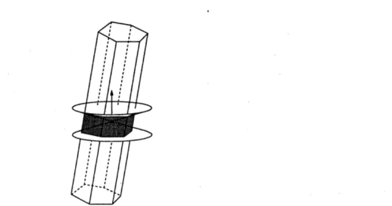
Well-sampled patch: Let $S\subseteq F$ be a surface patch such that each point $x\in S$ has

a

sample

within$\epsilon f(x)$ distance and$S$ ismaximal in the

sense

that

no

other point $y\not\in S$has this property.

Notice that $S$ may have several components. Boundaries of $S$ coincide with the boundaries of

undersampled regions in$F$

.

Ourgoal is to recognize the boundaries in$S$ and reconstruct it from

sample $P$

.

2.2

Boundaries

For any compact surface $S$ we can distinguish interior points from the boundary points. An

interior point has a neighborhood homeomorphic to the open disc$\mathrm{D}^{2}=\{x\in \mathbb{R}^{2} : |x|<1\}$

.

A

boundary point, on the other hand, has a neighborhood homeomorphic to the halfdisc $\mathrm{D}^{2}\cap \mathbb{P}_{+}$

which is openin the halfspace$\mathbb{P}_{+}=\{(x, y)\in \mathbb{R}^{2} : x\geq 0\}$.

For the reconstruction of$S$ only the finite set ofsample points$P$is given thatwell samples$S$

.

Even though all points in $P$ may be interiorpointsof$S$, the existence of

a

non empty boundary

should reflect itselfin the sample points. We are looking for

a

definition of interiorand boundary

pointsfor a finitesamplefrom asurface that captures theintuitive differencebetween interiorand

boundarypoints. We base

our

definition

on

the restricted Voronoidiagramasintroduced in [16].

Restricted Voronoi diagram: Let $P$ be

a

sample of

a

compact surface $S$ with

or

without

boundary embedded in $\mathbb{R}^{3}$

.

Denote the Voronoi diagram of _$P$ by _{$V_{P}$}. The restriction of _{$V_{P}$}

on the surface $S$ defines the restricted Voronoi diagram containing the restricted Voronoi cells $V_{p,S}=V_{p}\cap S$.

Thedualofthe restrictedVoronoidiagramdefinesthe restricted Delaunay triangulation$D_{P,S}$.

Specifically,

an

edge$pq$isin$D_{P,S}$iff$V_{p,S}\cap V_{q,S}=\emptyset$; a triangle_$pqr$is in$D_{P,S}$iff$V_{p,S}\cap V_{q,S}\cap V_{r,S}=\emptyset$

and

a

tetrahedron pqrs is in $D_{P,S}$ iff$V_{p,S}\cap V_{q,S}\cap V_{r,S}\cap V_{s,S}=\emptyset$. Edelsbrunner and Shah [16]

showed that ifeach restricted Voronoi cell (defined recursivelywith dimensions) is a closed ball,

andthe

same

conditionholdsforthe boundaryof$S$,then$S$ is homeomorphic to_{$D_{P,S}$}. This leads

us todefine the neighborhood ofa sample point$p$as $V_{p,S}$.

Using this definition of neighborhood

we

define interior vertices. All vertices that

are

not

Deflnition 1 (Interior and boundary vertices) A sample point$pfmm$ a sample $P$

of

$S$ is

called interior vertex

_if

$V_{p,S}$ does not contain a boundarypoint

of

S.

Samplepoints that

are

not

interior are called boundary vertices.

Arguments of

[1] can

be usedto show that the neighborhoods of interior vertices are

homeo-$\dot{1}$

morphic todisks if$P$is

an

$\epsilon$-sampleof$S$ with $\epsilon<0.1$

.

2.3

Flat

vertices

Ourgoal is to detect boundary vertices algorithmically and to exploit thisinformationfor surface

reconstruction.

Given

onlya finitesample$P$from

a

surface$S$embedded in$\mathbb{R}^{3}$

we

cannot construct

the restrictedVoronoidiagram$V_{P,S}$, becausethesurface$S$isunknowntous. Therefore wecannot

exploit

our

definitionofinteriorand boundaryverticesalgorithmically.

To cope with this problem

we

define

a

_flatness

condition and show that boundary vertices

cannot be flat whereas interior vertices with well sampled neighborhoods

are

flat. This definition

uses

the definitions ofpoles and the width and heights ofVoronoicells. The benefit weget from the definitionof flat vertices is that it canbe exploited algorithmically.

Ray: In$\mathrm{w}\mathrm{h}.\mathrm{a}\mathrm{t}\mathrm{f}\mathrm{o}\mathrm{l}\mathrm{l}\mathrm{o}\mathrm{w}\mathrm{s},\mathrm{w}\mathrm{e}$willdenote the$\mathrm{r}..\mathrm{a}\mathrm{y}$from$p$to$y\mathrm{w}$

.ith

$\vec{y}$for any

$\mathrm{s}\mathrm{a}\mathrm{m}\mathrm{p}\mathrm{l}\mathrm{e}$ point$p$

a.nd

any

point $y\in V_{p}$.

Angles: We usethe notation $\angle(v_{1}^{arrow}, v_{2}^{arrow})$ to denote the acute angle between the lines supporting

two vectors$v_{1}^{arrow}$ and $v_{2}^{arrow}$

.

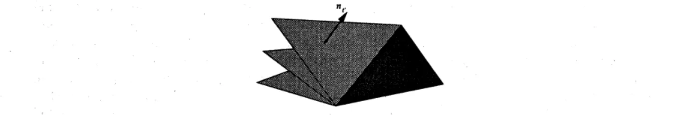
Poles: Given

a

finitepoint set $P\subset \mathbb{R}^{3}$, let

$V_{p}$ bethe Voronoicellof apoint_{$p\in P$}. We borrow

the definitionof poles from [1]. The vertex $v_{p}^{+}$ of the Voronoi cell $V_{p}$ which isfarthest from the

point$p$iscalled the positive pole of$V_{p}$. Assumingthat $P$does not lieon aplane,$v_{p}^{+}$ always exists.

The negative pole of $V_{p}$ is the farthest point $v_{p}^{-}\in V_{p}$ from$p$ such that $v_{p}arrow-$

.

$v_{p}arrow+<0$

.

Basically,

negative pole is thefarthest point in $V_{p}$ in the

“opp.o.site

direction” of the positive pole.

$Co$-cone: The set $C_{p}= \{y\in V_{p} : \angle(y^{arrow}, v_{p}^{\sim+})\geq\frac{3\pi}{8}\}$ is calledthe $\mathrm{c}\mathrm{o}$

-cone

of_$p$

.

Basically, $C_{\mathrm{p}}$ is

the complement of

a

double

cone

(clipped within$V_{p}$) centered at_$p$withan opening angle $\frac{3\pi}{8}$

.

See

Figure 1 foran example ofa

co-cone.

$Co$-cone neighbors: Givena finitesample $P$, the set $N_{p}=\{q\in P : C_{p}\cap V_{q}\neq\emptyset\}$is called the

set of$\mathrm{c}\mathrm{o}$

-cone

neighbors of

$p$.

Width and height

_of

Voronoi cells: The width$w(V_{\mathrm{p}})$of the Voronoicell$V_{p}$of$p$is definedas the

radiusof$C_{p}$, i.e.,_{$w(V_{p})= \max\{|py| : y\in C_{p}\}$},

see

alsoFigure1. Let_{$h^{+}(V_{p})$}and

$h^{-}(V_{p})$denotethe

lengths $|pv_{p}^{+}|$ of$v_{p}arrow+\mathrm{a}\mathrm{n}\mathrm{d}|pv_{p}^{-}|$ of$v_{p}arrow-\mathrm{r}\mathrm{e}\mathrm{s}\mathrm{p}\mathrm{e}\mathrm{c}\mathrm{t}\mathrm{i}\mathrm{v}\mathrm{e}\mathrm{l}\mathrm{y}$. Definethe height $h(V_{p})$ as $\min(h^{+}(V_{p}), h^{-}(V_{p}))$.

Now, we areprepared to define flatness, which depends on two parameters $\rho$ and $\theta$.

Definition 2 (Flatness) A sample point$p\in P$ is called

flat if

thefollowing two conditions hold:

1. Ratio condition: $\rho w(V_{p})\leq h(V_{\mathrm{p}})$

2. Normalcondition: $\forall q$ with$p\in N_{q},$ $\angle(v_{p}^{+}, v_{q}^{+})\leq\theta$.

Ratio condition imposes that the Voronoi cell $V_{p}$ is long and thin in the directions of the pole vectors$v_{\mathrm{p}}\mathrm{a}\mathrm{n}\mathrm{d}\wedge\vdash v_{p}arrow-$. Thenormal conditionstipulates thatthedirection ofelongationof

Figure 1: A Voronoi cell together with the normalized pole vector and the $\mathrm{c}\mathrm{o}$-cone (shaded).

with that of any vertex whose $\mathrm{c}\mathrm{o}$

-cone

neighbor is_$p$. In the proof

we use

$\rho=\frac{1}{1.3\epsilon}$ and $\theta=0.14$

radians.

3

Assumptions and Theorems

Ourgoal is to exploit the definitionofflat vertices in aboundarydetection algorithm. In Theorem

1we provethat interior vertices with well sampled neighborhoods

are

flat. In Theorem2we prove

that the boundary vertices cannot be flat. These two theorems form the basis of

our

boundary

detection algorithm. Weomit the proofsofthese two theorems inthis version. See[10] for details.

In the proofs we

assume

$\epsilon\leq 0.01,$ $\rho=\frac{1}{1.3\epsilon}$ and $\theta=0.14$ radians. With these values we

can

show that interior vertices satisfy the ratio condition. However, the normal condition may not

hold for all ofthem. Nevertheless, we can show that a subset ofinterior vertices that have well

sampled neighborhoods satisfy the normal condition. To be precise

we

introduce the following

definition.

Definition 3 (Deep interior vertex:) An interior vertex$p$ is called deep

if

it does not have

any boundary vertex as Voronoi neighbor.

Theorem 1 All deep interior vertices are

_flat.

For Theorem 2weneed

some

boundary assumptions. The first assumption (i)saysthat

bound-aryvertices remain as boundary evenif $S$ is expandedwith a small collar around its boundary,

and the assumption (ii) stipulates that the boundaries be “well separated”. Assumption 1 (Boundary assumption)

$i$. The restricted Voronoi cell

of

a boundary vertex is a disk. The

surface

patch $S’\supset S$ with

the condition that any$x\in S’$ has a sample within$\delta f(x)$ distance

for

some $\delta>\epsilon$

defines

the

same set

_of

boundaryvertices as$S$ does. We will need$\delta=1.3\Delta\epsilon$

for

ourproofs, where $\Delta$ is

defined

as $\max\{\frac{h(V)}{f(p)}\}$

.

$ii$

.

Neighborhood

of

each boundary vertex intersects the neighborhood

of

at least an interior

vertex.

Remark. It is interesting tonote that one

can assume

the surface$F$tohavesmallfeatures around

any sample point to render it

as a

boundary point in our definition. After all, the surface $F$ is

unknown to

us.

This should reflect inour assumptions and proofs. Observethat,the smaller the

feature size gets, the larger gets $\Delta$

as

_{$\Delta=\max\{\frac{h}{f(}Ep\overline{)}\}$}

.

In order forboundary assumption to be

valid, weneed $\delta$ to be fixed

even

though $\Delta$ increases. This requires $\epsilon$ to decrease as $\delta=1.3\Delta\epsilon$

.

But, decreasing $\epsilon$ would require alarger value

$\mathrm{o}\mathrm{f}\rho\wedge\cdot$ Thus, indeed larger valueof$\rho$

are

needed to

detect

more

vertices

as

boundary.

4

Boundary

detection

Thealgorithm for boundary detection first computes the set of interior vertices, $R$, that areflat.

It uses two parameters$\rho$ and

$\theta$ to check the ratio and normal conditions. In theory, we require $1\mathrm{a}\mathrm{r}\mathrm{g}\mathrm{e}\mathrm{T}\mathrm{h}\mathrm{e}\mathrm{o}\mathrm{r}\mathrm{e}\mathrm{m}1\mathrm{a}\mathrm{n}\mathrm{d}\mathrm{A}\mathrm{s}\mathrm{s}\mathrm{u}\mathrm{m}\mathrm{p}\mathrm{t}\mathrm{i}\mathrm{o}\mathrm{n}2\mathrm{g}\mathrm{u}\mathrm{a}\mathrm{r}\mathrm{a}\mathrm{n}\mathrm{t}\mathrm{e}\mathrm{e}\mathrm{t}\mathrm{h}\mathrm{a}\mathrm{t}R\mathrm{i}\mathrm{s}\mathrm{n}\mathrm{o}\mathrm{t}\mathrm{e}\mathrm{m}\mathrm{p}\mathrm{t}\mathrm{y}$

.

$\mathrm{I}\mathrm{n}\mathrm{a}\mathrm{s}\mathrm{u}\mathrm{b}\mathrm{s}\mathrm{e}\mathrm{q}\mathrm{u}\mathrm{e}\mathrm{n}\mathrm{t}\mathrm{p}\mathrm{h}\mathrm{a}\mathrm{s}\mathrm{e}R\rho=\frac{1}{1.3\epsilon,\mathrm{r}\theta}$

.

$\mathrm{a}\mathrm{n}\mathrm{d}\theta=0.14.\mathrm{H}\mathrm{o}\mathrm{w}\mathrm{e}\mathrm{v}\mathrm{e}\mathrm{r},\mathrm{i}\mathrm{n}\mathrm{o}\mathrm{u}\mathrm{r}\mathrm{i}\mathrm{m}\mathrm{p}\mathrm{l}\mathrm{e}\mathrm{m}\mathrm{e}\mathrm{n}\mathrm{t}\mathrm{a}\mathrm{t}\mathrm{i}\mathrm{o}\mathrm{n}\mathrm{w}\mathrm{e}\mathrm{o}\mathrm{b}\mathrm{t}\mathrm{a}\mathrm{i}\mathrm{n}\mathrm{g}\mathrm{o}\mathrm{o}\mathrm{d}\mathrm{r}\mathrm{e}\mathrm{s}\mathrm{u}\mathrm{l}\mathrm{t}\mathrm{s}\mathrm{f}\mathrm{o}\mathrm{r}\mathrm{s}\mathrm{m}\mathrm{a}\mathrm{l}\mathrm{l}\mathrm{e}\mathrm{r}\rho \mathrm{a}\mathrm{n}\mathrm{d}$

is expanded to include all interior vertices in aniterative procedure. A genericiteration proceeds

asfollows. Let$p$beany

co-cone

neighbor ofavertex$q\in R$

so

that$p\not\in R$and$V_{p}$ satisfiesthe ratio

condition. If$v_{p}^{+}$ and$v_{q}^{+}$ make smallangle up to orientation, i.e., if$\angle(v_{p}^{arrow+}, v_{q}^{arrow+})\leq\theta$,

we

include$p$

in $R$

.

Ifno such vertex

can

be found, the iteration stops. We arguethat $R$includes only and all

interior vertices at the end. The rest of the vertices are detected

as

boundary

ones.

Thefollowing routine$\mathrm{I}\mathrm{s}\mathrm{F}\mathrm{L}\mathrm{A}\mathrm{T}$ checks the conditions stated in Definition 2 to detect flat vertices.

The input isasample point$p\in P$with

a

parameter$\rho$that

measures

the height$\mathrm{v}\mathrm{s}$. width ratiofor

$V_{p}$

.

The return value is true if$p$is

a

flat vertex, and false otherwise. The routine BOUNDARY

uses

$\mathrm{I}\mathrm{s}\mathrm{F}\mathrm{L}\mathrm{A}\mathrm{T}$ to detectthe boundary vertices. $\mathrm{I}\mathrm{s}\mathrm{F}\mathrm{L}\mathrm{A}\mathrm{T}(p\in P, \theta, \rho)$

1 computethe width$w(V_{p})$ and the height$h(V_{p})$

2 if$\rho w(V_{p})\leq h(V_{p})$

3 if$\forall q$ with_{$p\in N_{q}$} : $\angle(v_{p}v_{q})\sim\vdash,arrow+\leq\theta$

4 return true

5 return false

BOUNDARY $(P, \theta, \rho)$

1 $R:=\emptyset$

2 for all$p\in P$

3 if$\mathrm{I}\mathrm{s}\mathrm{F}\mathrm{L}\mathrm{A}\mathrm{T}(p)R:=R\cup p$

4 while $\exists p\not\in R$and $\exists q\in R$with$p\in N_{q}$,

and $\rho w(V_{p})\leq h(V_{p})$ and $\angle(v_{p}^{+}, v_{q}^{+})\leq\theta$ $5$ $R:=R\cup p$

6 return $P\backslash R$

4.1

Justification

We

can

show that BOUNDARY computesall and only boundary vertices if

we

make the following

assumption. Notice thatthis assumption is valid formost practical data. The proofofthe claim

is available in [10].

Assumption 2 (Interior assumption) Each interiorvertexis path connectedto adeepinterior

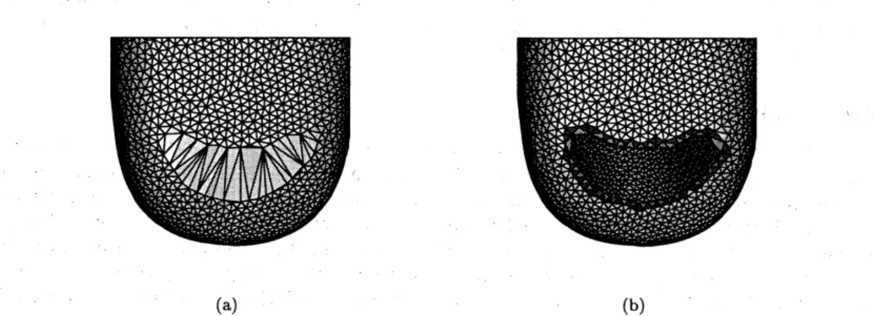
Figure 2 shows two triangulationsofthe dataset FOOT. The first triangulation

is

computed

with the

CO-CONE

algorithm [4] without boundary detection. The second triangulation is

com-puted with the modified CO-CONE algorithm that

uses

BOUNDARY to detect boundary vertices.

biangles incident to the boundary verticesare shaded darker.

(a) (b)

Figure 2: hiangulation of the dataset FOOT (a) without boundary detection; thebig hole above

the ankle iscovered with triangles, (b) with boundary detectionusing the algorithm BOUNDARY;

the hole above the ankle is well detected.

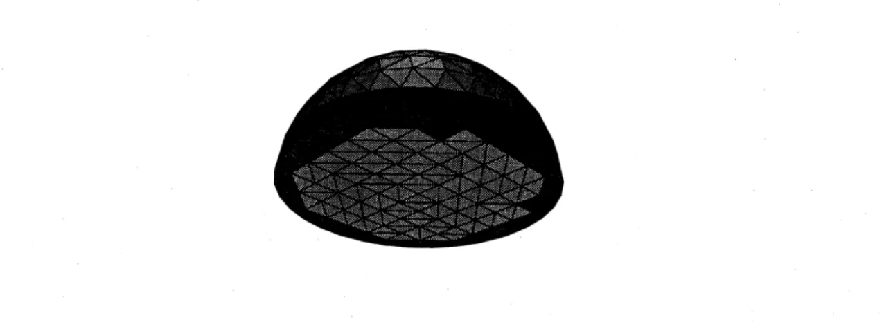
Non-smoothness

Recallthat

our

theoryis based

on

the assumption that the sampledsurface is smooth. However,

we

observe that the boundary detection algorithm also detectsundersamplingin non-smooth surfaces,

see

Figure3and also Figure 7,8and10. The ability to handle non-smoothsurfaces

owes

tothefact

thatnon-smooth surfacesmaybe approximatedwith asmooth

one

that interpolates the samples.

Forexample,

one can

resortto the implicit surfacethat is$C^{1}$-smooth and interpolates the sample

points using natural co–ordinates as explained in [8]. For higher order continuity results of [20]

can be called upon. These smooth surfaces have high curvatures

near

the sharp features of the

original non-smooth surface. Our theory

can

be applied to the approximating smoothsurface to

ascertainthat the samples in the vicinity of sharp features act asboundary vertices in the vicinity

of high curvatures forthe smooth surface.

Figure3: Boundaryvertices

are

detected inthevicinityofthe sharpedgein HALFSPHERE,triangles

5

Surface

reconstruction

Our

goal is to reconstruct

a

smooth compact surface $S\subset \mathbb{R}^{3}$ which may have

a

non-empty

boundary from

a

finite sample $P\subset S$

.

For this purpose

we

modify the $\mathrm{C}\mathrm{O}$-CONE algorithm [4]

such that it is capable ofreconstructing surfaceswith boundary. Like the

CRUST

the CO-CONE

algorithm consists of three steps:

(1)

CANDIDATETRIANGLEEXTRACTION.

In this step a set of candidate triangles forthe

recon-struction is extracted from the Delaunay triangulation of the sample points. In general the

underlyingspace ofthese triangles

_is.

not amanifold, but a manifoldwith boundary canbe

extracted in the next two steps.

(2) PRUNING. The candidate $\dot{\mathrm{t}}\mathrm{r}\mathrm{i}\mathrm{a}\mathrm{n}\mathrm{g}\mathrm{l}\mathrm{e}\mathrm{s}$

are

already close to a manifold for sufficiently dense

samples. Wewant to extract a manifold fromthis set by walking

on

the outsideorinsideof

this set. During the walk

we

may encounter the problemofentering

a

triangle $t$ which has

abareedge, i.e., anedge incident toasingle triangle, namely $t$. The purpose of this step is

toget rid of these edges with their incident triangles.

(3) WALK. We walk on the out- or inside of the set of triangles that remained after pruning

and report the triangles walked

over.

We modify the first step of CO-CONE algorithm for boundary detection. In the original

co-cone

algorithm each sample chooses a set of candidate triangles incident to it. In the modified

algorithm, only the interior verticesare allowed to choose the candidate triangles.

CANDIDATETRIANGLEEXTRACTION $(P\subset \mathbb{R}^{3}, \theta\in(0, \pi/2), \rho)$

1 compute the Voronoi diagram$V_{P}$

2 $CandidateTriangles:=DelaunayTriangles$

3 $B:=\mathrm{B}\mathrm{o}\mathrm{u}\mathrm{N}\mathrm{D}\mathrm{A}\mathrm{R}\mathrm{Y}(P, \theta, \rho)$

4 for each sample$p\in P$

5 if$p\not\in B$ .

6 for eachVoronoi edge $e\in V_{p}$

7 if$C_{p}\cap e\neq\emptyset$

8 e.Mark.insert$(p)$

.

$\mathrm{v}$

9 for each Voronoi edge$e\in V_{P}$

10 for each$p\in \mathrm{D}\mathrm{u}\mathrm{A}\mathrm{L}\mathrm{T}\mathrm{R}\mathrm{I}\mathrm{A}\mathrm{N}\mathrm{G}\mathrm{L}\mathrm{E}(e)\cap P$

11 if$(p\not\in B)$ and $(p\not\in e.Mark))$

12 CandidateTriangles.delete$(\mathrm{D}\mathrm{u}\mathrm{A}..\iota \mathrm{T}\mathrm{R}\mathrm{I}\mathrm{A}\mathrm{N}\mathrm{G}\mathrm{L}\mathrm{E}(e))-$

13 return CandidateTriangles

First the set CandidateTriangles is initialized to the set ofall Delaunay triangles (line 2).

This set getsfilteredsubsequently. EachVoronoiedge$e$has

a

fieldMark that collects the samples

whose$\mathrm{c}\mathrm{o}$

-cones

intersect$e$ (line 7). This check is done only if the sample is notaboundary vertex.

In otherwords, only interior vertices mark the Voronoiedges that intersect their$\mathrm{c}\mathrm{o}$-cones. Next,

we look at the markings of theVoronoi edges and delete their dual triangles from the candidate

set if they

are

not marked by an adjacent sample which is interior (lines 10-12). In essence, we

rely only

on

thetriangles that

are

chosen by interior vertices and

a

triangle is in the candidate set

onlyifallofits interior vertices have chosen it.

Thesecond step PRUNING

removes

triangles incident to sharp edges ina cascaded manner

as

was

originally suggested in [1]. An edge $e$ is called sharp if there are two consecutive triangles

if it has only

one

incident triangle. Wehave to be carefulin this stepnot totrigger the cascaded

deletion ofthe desired surface by deleting

a

triangle incident

on a

boundary vertex which has

a

bareedge. So,

we

remove a

triangle only if it isnot incident

on a

boundary vertex.

Let $K$ be atwo dimensionalsimplicialcomplex.

PRUNING $(K)$

1 Pending:$=\emptyset$

2 for each edge $e\in K$

3 Pending.push$(e)$

4 while Pending$\neq\emptyset$

5 $e:=Pending.pop()$

6 if$\mathrm{I}\mathrm{s}\mathrm{S}\mathrm{H}\mathrm{A}\mathrm{R}\mathrm{P}(e)=\mathrm{t}\mathrm{r}\mathrm{u}\mathrm{e}$

7 for each $t\in e.Triangles$

8 if$\forall(p\in t\cap P)p\not\in B$

9 $K:=K\backslash \{t\}$

10 for each $e’\in t.Edges\backslash \{e\}$

11 Pending.push$(e’)$

12 return $K$

Firstastack Pending isinitialized empty (line 1). Then alledges in the complex$K$arepushed

onto this stack (lines 2 and 3). Together with everytriangle$t$

we

storea list Edges ofits edges.

With each edge $e$ we store a set Triangles of triangles incident to $e$

.

We assume that we have

afunction $\mathrm{I}\mathrm{s}\mathrm{S}\mathrm{H}\mathrm{A}\mathrm{R}\mathrm{P}$ available that requires an edge _$e$

as

input and returns trueif

$e$ is sharp and

false if $e$ is not sharp. As long

as

the stack Pending is not empty, an edge $e$ is popped from

the stack. If this edge is sharp, allthoseincident triangles

are

removedfrom the complex$K$that

are

not incident to a boundary vertex. All edges other than $e$ that are incident to the deleted

triangle$t$arepushed onto the stack Pending (lines 4–11). These edges maybecome sharp due

to the deletion of the triangle $t$. Observe that during deleting triangleswe not only check if it

is incident to a sharp edge, but also check if it is incident to any boundary vertex. Finally, the

reduced complex$K$ is returned (line 12).

The third step WALK extracts amanifold.

WALK $(K)$

1 Sur

_face

$:=\emptyset$

2 choose arbitrary oriented$t\in K$

3

_{Surface.insert}

$(t)$

4 Pending:$=\emptyset$

5 for each $earrow\in t.Edges$

6 Pending.push$((e, tarrow))$

7 while Pending $\neq\emptyset$

8 $(etarrow,):=Pending.pop()$

9 if e.processed$=\mathrm{f}$alse

10 e.processed:$=\mathrm{t}\mathrm{r}\mathrm{u}\mathrm{e}$

11 $t’:=\mathrm{S}\mathrm{u}\mathrm{R}\mathrm{F}\mathrm{A}\mathrm{C}\mathrm{E}\mathrm{N}\mathrm{E}\mathrm{I}\mathrm{G}\mathrm{H}\mathrm{B}\mathrm{O}\mathrm{R}(K, etarrow,)$

12 if$t’\neq\emptyset$

13

_{Surface.insert}

$(t’)$

14 foreach $e^{\neg}\in t’.Edges\backslash \{e\gamma$

15 Pending.push$((et’\neg,))$

First

we

initialize theset

_Surface

empty (line 1). Then

we

choose

an

arbitrary triangle$t$from

the complex $K$, orient it and insert it in the the set

Surface

(lines 2 and 3). Next

we

initialize

the stack Pending empty (line 4). From the orientation of the chosen triangle $t$ we derive

an

orientation for all edges incident to $t$

.

These edges

are

stored in

a

field Edges associated with

every triangle. We denote an oriented edge $e$ by $earrow$

.

For each oriented edge

$e$ oftriangle $t$, we

pushthe pair $(etarrow,)$ onto the stack (lines 5 and 6). As longasthe stack Pending is not empty,we

popits top element $(etarrow,)$ (line8). If the edge$e$ is not processed

so

far we usethe fieldprocessed

to mark it processed and compute the surface neighbor of $(etarrow,)$, i.e. the triangle $t’$ incident to $e$

that ‘best fits’ $t$ (lines 9-11). If$t’$ does not exist, the triangle $t$ is incident to the boundary. We

insert $t’$ in the set

Surface

(lines 12 and 13). We

assume

that the function $\mathrm{S}\mathrm{u}\mathrm{R}\mathrm{F}\mathrm{A}\mathrm{C}\mathrm{E}\mathrm{N}\mathrm{E}\mathrm{I}\mathrm{G}\mathrm{H}\mathrm{B}\mathrm{O}\mathrm{R}$

orients$t’$ such that its orientationmatches the orientation of$t$ andpush all the pairs oforiented

edges$e^{\neg}$ besides $e\mathrm{i}arrow \mathrm{n}\mathrm{c}\mathrm{i}\mathrm{d}\mathrm{e}\mathrm{n}\mathrm{t}$to $t’$ together with the triangle $t’$ itself onto the stack Pending (lines

14and 15). Finallywereturnthe surface

_Surface

(line 16). The above method works under the

assumptionthat thesurface is orientable, i.e., surfaceslikeM\"obius strip

are

not allowed.

The return value $t’$ of$\mathrm{S}\mathrm{u}\mathrm{R}\mathrm{F}\mathrm{A}\mathrm{C}\mathrm{E}\mathrm{N}\mathrm{E}\mathrm{I}\mathrm{G}\mathrm{H}\mathrm{B}\mathrm{O}\mathrm{R}(C, etarrow,)$is the topmost triangle triangleamong the

set oftriangles incident to$e$ whosenormals (oriented according to the orientationof$t$) make

an

angle smaller than $\frac{\pi}{2}$ with thenormal of$t$,

see

Figure 4.

Figure 4: The surface neighbor ofthe dark grey shaded triangle is the topmost triangle among

thelight grey shaded triangles.

Putting the three steps CANDIDATETRIANGLEEXTRACTION, PRUNING and WALK together

gives the modified

CO-CONE

algorithm.

CO-CONE $(P\subset \mathbb{R}^{3}, \theta\in(0, \pi/2), \rho)$

1 $K:=\mathrm{C}\mathrm{A}\mathrm{N}\mathrm{D}\mathrm{I}\mathrm{D}\mathrm{A}\mathrm{T}\mathrm{E}\mathrm{T}\mathrm{R}\mathrm{I}\mathrm{A}\mathrm{N}\mathrm{G}\mathrm{L}\mathrm{E}\mathrm{E}\mathrm{x}\mathrm{T}\mathrm{R}\mathrm{A}\mathrm{C}\mathrm{T}\mathrm{I}\mathrm{O}\mathrm{N}(P, \theta, \rho)$

2 $K’:=\mathrm{P}\mathrm{R}\mathrm{U}\mathrm{N}\mathrm{I}\mathrm{N}\mathrm{G}(K)$

3 $K”:=\mathrm{W}\mathrm{A}\mathrm{L}\mathrm{K}(K’)$

4 return$K”$

6

Implementation and results

As with many other geometric algorithms we faced the numerical robustness as an important

issue in implementing CO-CONE. There

are

two main

sources

of problems. First, algorithms

and data structures defined under

a

general position assumption do not workfor practical data

sets since such degenerate situationsdo

occur.

Second,

we

need toevaluate geometric predicates

which

are

difficult to compute exactly (especiallyifthesituation is close to

a

degenerateone). To

copewith this problem

we

resort to the robust library of geometric algorithms called

CGAL

[24]

code whichmakes it easy to

use

different numbertypes and implementationsofpredicates for the computation.

For

our

implementation ofthe CO-CONE algorithm

we

usedthe Delaunaytriangulation from

the

CGAL

library togetherwith filteredpredicates. Computation of filteredpredicatessimulates

exact evaluation

on a

demand basis and thus

runs

faster than predicate evaluations with exact arithmetic. Instead of filtered predicates if we

use

floating point arithmetic the running time

decreasesroughly by a factor oftwo,

see

Table 2. However, results maynot bereliable.

Besides robustness we encountered a problem whichis

more

inherent to our algorithm: Some

datacontain noise beyond the toleranceofthe CO-CONE algorithm. Thismayturn

some

interior vertices

as

“false boundary vertices”. These points

are

detected as interior by BOUNDARY, but

their incident candidate triangles after the CO-CONE step do not form

a

flat disk. Thus, the

pruning step

runs

the risk ofdeleting the desired output since it does not recognizethese “false

boundary vertices”. That means, it can happen that during the PRUNING step all triangles are

removes

that

are

not incident to a boundary vertex. To cope with this problem,

we

employ a

safety check$\mathrm{H}\mathrm{A}\mathrm{s}\mathrm{U}\mathrm{M}\mathrm{B}\mathrm{R}\mathrm{E}\mathrm{L}\mathrm{L}\mathrm{A}$ toeach vertex.

6.1

Umbrella

check

An umbrella incidentto

a

vertex$p\in K$ isasetoftrianglesincident to$p$whichform

a

topological

closed disc $\mathrm{I}\wp$

.

An umbrella is called sharp if it contains a sharp edge. $\mathrm{H}\mathrm{A}\mathrm{s}\mathrm{U}\mathrm{M}\mathrm{B}\mathrm{R}\mathrm{E}\mathrm{L}\mathrm{L}\mathrm{A}$ deletes

the sharp edges and their incident triangles in

a

cascaded

manner.

But, unlike pruning this

cascaded deletion is applied only to edges and triangles incident to the vertex being checked.

If the vertex retains a triangle after this cascaded deletion, $\mathrm{H}\mathrm{A}\mathrm{s}\mathrm{U}\mathrm{M}\mathrm{B}\mathrm{R}\mathrm{E}\mathrm{L}\mathrm{L}\mathrm{A}$ returns true. To

avoidmisunderstandings note that $\mathrm{H}\mathrm{A}\mathrm{s}\mathrm{U}\mathrm{M}\mathrm{B}\mathrm{R}\mathrm{E}\mathrm{L}\mathrm{L}\mathrm{A}$

removes

the triangles only virtually, i.e. after

applying $\mathrm{H}\mathrm{A}\mathrm{s}\mathrm{U}\mathrm{M}\mathrm{B}\mathrm{R}\mathrm{E}\mathrm{L}\mathrm{L}\mathrm{A}$ to

a

point _$p$ of

a

complex$K$the set oftriangles incidentto$p$ is exactly

the

same

asit

was

before. That means, $\mathrm{H}\mathrm{A}\mathrm{s}\mathrm{U}\mathrm{M}\mathrm{B}\mathrm{R}\mathrm{E}\mathrm{L}\mathrm{L}\mathrm{A}$ is only used tocheckif

a

point has a

non

sharp umbrellabut not to alter the complex$K$

.

$\mathrm{H}\mathrm{A}\mathrm{s}\mathrm{U}\mathrm{M}\mathrm{B}\mathrm{R}\mathrm{E}\mathrm{L}\mathrm{L}\mathrm{A}(K, p\in K)$

1 Umbrella:$=p.Triangles$

2 Pending$:=\emptyset$

3 for everyedge $e\in p.Edges$

4 Pending.push$(e)$

5 whilePending $\neq\emptyset$

6 $e:=Pending.pop()$

7 if $\mathrm{I}\mathrm{s}\mathrm{S}\mathrm{H}\mathrm{A}\mathrm{R}\mathrm{P}(e)=\mathrm{t}\mathrm{r}\mathrm{u}\mathrm{e}$

8 for each $t\in e.Triangles$

9 Pending.push$(t\cap(p.Edges\backslash e))$

10

Umbrella.delete

$(t)$

11 ifUmbrella$=\emptyset$

12 return false

13 return true

First the set Umbrella is initialized to the set of triangles incident to $p$ (line 1). Next

we

initializethe stackPending empty (line 2). Then wepush all edges $e$incidentto$p$ontothe stack

Pending (lines 3 and4). We

assume

that the edges incident to$p$

are

storedinthe set Edges and

the triangles incident to$p$

are

stored in the set Triangles. As long

as

the stackPending is not

empty

we

popits top element. If this elementis asharpedge$e$, we delete alltrianglesincident to

$e$inthe complex$K$fromthe set Umbrella,andpush alledgesincident tosuch

a

triangle and the

point$p$besidesthe edge $e$onto the stackPending (lines 5-11). Finally

we

return false ifthe set

The boundaryverticesdetected by

our

implementation

are

the unionofthe boundaryvertices

detected by the algorithm BOUNDARY and the vertices not detected by the algorithm

HASUM-BRELLA. Weobserve that PRUNING with this enlarged setofboundary vertices issafe. Forsamples

fromsmooth surfaces that fulfill the sampling conditionweobservethatUMBRELLACHECKis not

necessary.

6.2

Parameters and precision

In the proofs wechoose the ratio $\rho$ ofthe height to the width of

a

Voronoi cell to be

more

than

$\frac{1}{1.3\in}$

.

In practiceavalue between 1.1 and 1.7gives good results. Increasing this ratio detectsmore

pointsas boundaryas can be observed in Figure5.

(a) (b)

Figure 5: Both figures show the reconstructed heel of the dataset FOOT fordifferent values of$\rho$

.

In (a) this ratio is 1.5 and in (b) it is

4.3.

Although$\theta$is0.14radians in theory,avalueaslargeas

$\frac{\pi}{6}$ gives good results. We observed that

the output is quite sensitive to the opening angleofthe double

cones

that defines$\mathrm{c}\mathrm{o}$

-cones.

If this

angle is decreased, the width increases with the inverse of the $\sin$of this angle. Thus, the height

$\mathrm{v}\mathrm{s}$

.

width ratio deteriorates quite sharply forcing the ratio condition fail for many vertices. On

the other hand, ifwemake this angle larger $\mathrm{c}\mathrm{o}$-cones become thinnerwhich may not allow some

of the desired triangles to be captured

as

candidate triangles. We used $\frac{3\pi}{8}$ to define the

co-cones

both in theory and practice.

Asmentioned earlier, numerical robustness isanimportant issue inourreconstruction software.

Figure6 shows the reconstructionfor the dataset HALFSPHERE withfloating point arithmetic and

with filtered exact arithmetic. Numerical problem

occurs

in this dataset since it contains many

$\mathrm{c}\mathrm{o}$-planar points causing degeneracies in the Delaunay triangulation. As

a

result the Delaunay

triangulation is computed incorrectly. CO-CONEtakes 1.9 seconds computing time with floating

point arithmetic compared to3seconds withfilteredpredicates. Figure 7shows the effectofusing

filtered predicates instead of floating point arithmetic for the OILPUMP dataset. Floating point

arithmetic takes 469 seconds for the reconstruction whereas filtered exact arithmetic takes 966

seconds. Considering the tradeoff between

running.

time and robustness

our

experiments show

that oneshould accept increased running time for reliable computations.

6.3

More datasets

We have experimented with many other datasets,

some

ofwhich

are

listed below. In the figures

(a) (b)

Figure6: Left and right figures show the reconstructed HALFSPHERE with floating point and exact

arithmetic respectively.

(a) (b)

Figure7: Reconstruction of the dataset OILPUMP (a) withfloating point arithmetic and (b) with

filteredexact arithmetic; sharpfeatures

are..

well detected.

The dataset ENGINE has three connected components. CO-CONE nicely $\mathrm{s}\mathrm{e}\mathrm{p}\mathrm{a}\mathrm{r}\mathrm{a}\mathrm{t}\mathrm{e}\mathrm{s}\vee$ the three

connected components and identifies the boundaries of the two outer shells. It alsoidentifies the

sharp tip of the innermost component,

see

Figure8.

Thedataset

CAT:

This dataset contains

a

single boundary at thebottom of the cat and

some

undersampled regions, especially at theears andlegs. Figure9 showsthe detected boundary and

undersampledregions.

Figure9: Thedataset CAT.

The dataset KNUCKLE: This is a challenging dataset for reconstruction, because it contains

many undersampledparts. This undersampling is mostly due to sharp features. Figure 10 shows

how the CO-CONE algorithm deals with undersampling. Most of the sharp features

are

well

detected. Tworegionswhereundersampling is extreme

are

shown with a

zoom.

(a) (b) (c)

Figure10: Reconstruction ofthe dataset KNUCKLE. In (a) theentire reconstructionis shown and

in (b) and (c) two undersampled parts

are

zoomed.

The dataset MANNEQUIN: Thisdataset contains oneboundary at the bottom and

undersam-pled regions in eyes, lips and

ears.

Figure 11 shows the reconstruction of this dataset with and

without boundary detection. Using boundary detection the CO-CONE detects the boundary at

the bottom

as

expected.

The dataset MONKEY: This dataset is created using the function $(x, y)-\neq x^{3}-3xy^{2}$

on

the

unit square. The graph of this function is called monkey saddle. The monkey saddle contains

a

single boundary which is perfectly detected. Figure 12 shows the monkey saddle and compares

(a) (b)

Figure 11: Reconstructionof the dataset MANNEQUIN (a)with boundary detection and(b)without

boundary detection.

(a) (b)

Figure 12: Reconstructionof the dataset MONKEY (a) with boundary detection and (b) without

boundarydetection.

6.4

Running

times

Wetested the CO-CONEalgorithm

on

many datasets. Allthe tests

were

done on

a

Silicon Octane

computer with 300 Mhz MIPS processor and 512 MByte ofmain memory. For all datasets we

used$\rho=1.5$ and $\theta=\frac{\pi}{6}$ in thealgorithm BOUNDARY.

For renderingweused Geomview [17], provided by the Geometry Center at the University of

Minnesota.

The basic data ofour experiments

are

summarized in Table 1. The running times are with

respect to filtered exact arithmetic. Observethat in all

cases

the numberof triangles is roughly

twice the number of points, which is expected from Euler’s formula.

Table 2 allows a closer look on the running times. We also included the timings when using

floatingarithmetic.

Since

the

CO-CONE

algorithm is logicallysplitinto threesteps: Delaunay triangulation, Bound-ary detectionand

_Surface

reconstru$c$tion

we measure

the CPU times foreach ofthese three steps.

As expected the Delaunay triangulation computation is the most time consuming step. The

running times usingfiltered arithmetic

are

almost twice

as

high

as

therunning times usingfloating

point arithmetic, but they

are

still in

a

reasonable range. The total running time shows

a

sub

object number of points number of triangles running time(sec.) $\ovalbox{\tt\small REJECT}_{0^{\mathrm{O}\mathrm{N}\mathrm{K}\mathrm{E}\mathrm{Y}}}\mathrm{M}\mathrm{A}\mathrm{N}\mathrm{N}\mathrm{E}\mathrm{Q}\mathrm{U}\mathrm{I}\mathrm{N}1277221\mathrm{K}\mathrm{U}\mathrm{N}\mathrm{C}\mathrm{K}\mathrm{L}\mathrm{E}601407912085243374\mathrm{M}10000196001620\mathrm{E}\mathrm{N}\mathrm{G}\mathrm{I}\mathrm{N}\mathrm{E}11360223561040\mathrm{F}\mathrm{o}\mathrm{O}\mathrm{T}2002139997592\mathrm{I}\mathrm{L}\mathrm{P}\mathrm{U}\mathrm{M}\mathrm{P}3093361041966\mathrm{C}\mathrm{A}\mathrm{T}1000019826311$

Table 1: Experimental data.

object Delaunay Boundary Reconstruction

$\ovalbox{\tt\small REJECT}_{0^{\mathrm{O}\mathrm{N}\mathrm{K}\mathrm{E}\mathrm{Y}}}\mathrm{M}\mathrm{A}\mathrm{N}\mathrm{N}\mathrm{E}\mathrm{Q}\mathrm{U}\mathrm{I}\mathrm{N}135- 57136- 77103- 77\mathrm{K}\mathrm{N}\mathrm{U}\mathrm{C}\mathrm{K}\mathrm{L}\mathrm{E}107- 4260- 3441- 45\mathrm{M}1328- 175- 117- \mathrm{E}\mathrm{N}\mathrm{G}\mathrm{I}\mathrm{N}\mathrm{E}836- 405107- 5897- 59\mathrm{F}\mathrm{o}\mathrm{O}\mathrm{T}233- 99224- 119138- 103\mathrm{I}\mathrm{L}\mathrm{P}\mathrm{U}\mathrm{M}\mathrm{P}414- 154313- 172239- 143\mathrm{C}\mathrm{A}\mathrm{T}121- 50108- 5882- 51$

Table 2: Acloser lookonthe running time of the CO-CONE algorithm in seconds. The first times

(before ‘-,) arewith respect tofiltered arithmetic and the second times (after ‘-,) arewith respect

tofloating point arithmetic. (Forthe MONKEY dataset the CGAL codewas not able to compute

the Delaunay triangulation using floating point arithmetic).

7

Conclusions

In thispaperwepresent analgorithm to detect the regions of undersampling in data that

are

sam-pledfromsomesurface. Thisprovidesa unified approachto reconstructsurfaces with boundaries

and to identify theregions of non-smoothnessorhigh curvature where undersampling doesoccur.

The existing algorithms with theoretical guarantees fail miserably on such data sets since they

assume that the data is derived from a smooth surface without any boundary. As exhibited by

our empirical results, our boundary detection algorithm correctly identifies the vertices that are

visiblylyingonthe boundary. Also, itidentifies the regions of non-smoothness and high curvature

effectively in practice.

Aprobablefollowup of this work is to investigatehowthis algorithm

can

be used to reconstruct

non-smoothsurfaces. After detecting the regions ofnon-smoothness,

can

werepair the surfaceto

fill up the “holes”? Currently research onthis question is under progress.

References

[1] N.Amentaand M. Bern. Surfacereconstruction byVoronoifiltering. Discr. Comput. Geom.,

22, (1999),481-504.

$.[2]$ N. Amenta, M. Bern and D. Eppstein. The crust and the $\beta$-skeleton: combinatorial curve

[3] N. Amenta, M. Bern and M. Kamvysselis.A new Voronoi-based surface reconstruction

algo-rithm.

SIGGRAPH

98, (1998), 415-421.

[4] N. Amenta, S.Choi, T. K.Deyand N. Leekha. A simplealgorithm for homeomorphicsurface

reconstruction. Proc. 16th. $ACM$Sympos. Comput. Geom., _(2000), 213-222.

[5] D. Attali.$r$-regular shape reconstructionfrom unorganized points. Proc. 13th$ACM$Sympos.

Comput. Geom., (1997),248-253.

[6] C. Bajaj, F. Bernardini and G. Xu. Automatic reconstruction of surfaces and scalar fields

from $3\mathrm{D}$ scans. SIGGRAPH95, (1995), 109-118.

[7] J. D. Boissonnat. Shape reconstruction from planar cross-sections. Computer Vision,

Graph-ics, and Image Processing 44 (1988), 1-29.

[8] J. D. Boissonnat and F. Cazals. Smoothsurface reconstruction via natural neighbor

interpo-lation of distance functions. Proc. 16th. $ACM$Sympos. Comput. Geom., (2000), 223-232.

[9] B. Curless and M. Levoy. A volumetric method for building complex models from range

images.

SIGGRAPH

96, (1996), 303-312.

[10] T. K. Dey and J. Giesen. Detecting undersampling in surface reconstruction. manuscript,

2000.

[11] T. K. Dey and P. Kumar. A simple provable algorithm forcurvereconstruction. Proc.

ACM-SIAMSympos. Discr. Algorithms, (1999), 893-894.

[12] T. K. Dey, K. Mehlhorn and E. A. Ramos. Curve reconstruction: connecting dots with good

reason. Comput. Geom. Theory Appl., 15, 229-244.

[13] T. K. Dey and R. Wenger. Reconstructingcurveswith sharp

corners.

To appear in 16th$ACM$

Sympos. Comput. Geom., 2000.

[14] H.Edelsbrunner. Shape reconstruction with Delaunay complex. LNCS1380, LATIN’98:

The-oretical

_Informati

$cs$, (1998), 119-132.

[15] H. Edelsbrunner and E. P. M\"ucke. Three-dimensional alpha shapes. $ACM$ Trans. Graphics,

13, (1994), 43-72.

[16] H. Edelsbrunner and N. Shah. Triangulating topological spaces. Proc. 10th $ACM$ Sympos.

Comput. Geom., (1994),285-292.

[17] $\mathrm{h}\mathrm{t}\mathrm{t}\mathrm{p}://\mathrm{w}\mathrm{w}\mathrm{w}.\mathrm{g}\mathrm{e}\mathrm{o}\mathrm{m}\mathrm{v}\mathrm{i}\mathrm{e}\mathrm{w}.\mathrm{o}\mathrm{r}\mathrm{g}$

[18] J. Giesen. Curvereconstruction, the TSP, and Menger’s theorem onlength. Proc. 15th$ACM$

Sympos. Comput. Geom., (1999), 207-216.

[19] C. Gold. Crust and anti-crust: aone-step boundaryand skeleton extraction algorithm. 15th.

$ACM$Sympos. Comput. Geom., (1999), 189-196.

[20] H. Hiyoshi and K. Sugihara. Voronoi-basedinterpolationwith higher continuity. Proc. 16th.

$ACM$Sympos. Comput. Geom., (2000), 242-250.

[21] H. Hoppe, T. $\mathrm{D}\mathrm{e}\mathrm{R}\mathrm{o}\mathrm{s}\mathrm{e}$, T. Duchamp, J. $\mathrm{M}\mathrm{c}\mathrm{D}\mathrm{o}\mathrm{n}\mathrm{a}\mathrm{l}\mathrm{d}$ and W. Stuetzle. Surface reconstruction

[22] M. Melkemi. $A$-shapes and their derivatives. lSth $ACM$

Sym.

pos. Comput.

Geom. ,

(1997),

367-369.

[23] D. Zorin andP. Schr\"oder. Subdivision formodeling and animation.

SIGGRAPH

99 Course Notes..