Length parameters for Teichmuller space of punctured surfaces(Complex Analysis on Hyperbolic 3-Manifolds)

(1)

Length parameters for Teichm\"uller space of punctured surfaces

by Toshihiro Nakanishi and Marjatta N\"a\"at\"anen

中西敏浩

1. Introduction

Let $F$ be the oriented closed surface of genus $g$ and $P$ a set of

$s$ points of $F$. The condition

$2g-2+s>0$

is assumed throughout

this paper. The Teichmuller space $T_{g,s}$ is the set of marked surfaces

with complete hyperbolic metric of finite area whose underlying topological

surface is $F\backslash P$. If an injective map $f$ : $T_{g,s}arrow R^{d}$ for some $d\geq 0$ is given, then $f$ gives a global parametrization for the space $T_{g,s}$. Among

several global parametrizations, the one by the geodesic length functions is well known ([4],[7],[8],[9], [10],[11]).

In case $P=\{x_{1}, \ldots, x_{s}\}$ is non-empty, there are other

parametriza-tions originally introduced by R. C. Penner for the decorated Teichm\"uller

space ([6]); If an ideal triangulation ofthe punctured surface $F\backslash P$ is given,

then the $h$-length coordinates and $L$-length coordinates associated with it

give global parametrizations for the Teichm\"uller space $T_{g,s}$ (for the

termi-nology, see Section 2. We remark that the $L$-length differs from Penner’s

$\lambda$-length by a constant factor.) The advantage of the parametrization by

$L$-length coordinates (or the $h$-length coordinates) is that it allows _{$T_{g)s}$}

a real-algebraic representation determined by comparatively simple equa-tions. The representation by the $L$-lengths is found in [3]. In terms of

the $h$-lengths, the representation of _{$T_{g,s}$} is described by $s$ equations

and $6g-6+3s$ so-called coupling equations whose geometric meanings are

almost trivial. In Section 2 we construct $L$-and $h$-length coordinates

associated with a special ideal triangulation and give the representations of

$T_{g,s}$.

In Section 3 we establish a relation between the $L$-lengths of ideal

arcs and the lengths of closed geodesics on a punctured hyperbolic surface and obtain an explicit real-algebraic representation of $T_{g,s}$ by geodesic

length functions.

In Section 4 we present a changing rule from the $h$-length coordinates

defined in Section 2 to the Fricke coordinates, that is, entries of the marked canonical generators (each is a$,$

$2\cross 2$ matrix) of the Fuchsian group

cor-responding to the point of $T_{g,s}$. This supplies another proof of the fact

(2)

Teichm\"uller space $T_{g,s}$.

2. Coordinates for the Teichm\"uller space associated with an ideal triangulation of a punctured surface

2.1. In this paper we employ the upper half plane model $H$ with

the metric $|dz|/({\rm Im} z)$ as the hyperbolic plane. Let $c$ be a complete

hyperbolic line. Then $c$ has two endpoints $v_{a},$$v_{b}$ in the boundary $\partial H$

of $H$ viewed as a subregion of the Riemann sphere. Choose horocycles

$C_{a}$ and $C_{b}$ based at $v_{a}$ and $v_{b}$, respectively. Let

$l$ denote the

signed distance between $C_{a}$ and $C_{b}$ along $c$, taken with positive sign if

$C_{a}\cap C_{b}=\emptyset$ and with negative sign if $C_{a}\cap C_{b}\neq\emptyset$. We call $e^{l/2}$ the

L-length of $c$ between $C_{a}$ and $C_{b}$ and denote it by $L(c;C_{a}, C_{b})$.

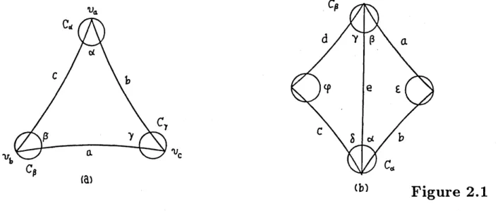
Let $T$ be a hyperbolic surface bounded by three complete lines. We

say that $T$ is an ideal triangle if $T$ has a finite area which necessarily

equals $\pi$. An ideal triangle has three ends. If an ideal triangle $T$ is

embedded in $H$, then the ends determine three vertices in $\partial H$. We adopt

the notation in Figure 2.1 (a). Suppose that a horocycle $C_{\alpha}$ based at

$v_{a}$

is given. We call the hyperbolic length of the part of $C_{\alpha}$ between the

edges $b$ and $c$ the h-length of the end $\alpha$ with respect to the horocycle

$C_{\alpha}$ and denote it by $h(\alpha, C_{\alpha})$.

For the ideal triangle $T$ equipped with horocycles as in Figure 2.1 (a),

the $L$-lengths of the edges and $h$-lengths of the ends associated with the

horocycles are related as in the following formulae:

(2.2)

$h( \alpha, C_{\alpha})=\frac{L(a;C_{\beta},C,)}{L(b;C_{7},C_{\alpha})L(c;C_{\alpha},C_{\beta})}$ $L(a;C_{\beta}, C_{7})= \frac{1}{\sqrt{h(\beta,C_{\beta})h(\gamma,C_{\gamma})}}$

2.3. Coupling equations. Consider a hyperbolic quadrilateral

which is cut into two ideal triangles by a diagonal. We adopt the no-tation of Figure 2.1 (b). Then the $h$-lengths of the ends which abut on the

diagonal $e$ satisfy the following coupling equation:

(3)

This equation follows easily from (2.2) if the expression of the $L$-length of $e$ in terms of the $h$-lengths is considered in each of the two triangles.

$(\mathfrak{y})$

Figure 2.1 2.5. Let $R$ be a hyperbolic surface with finite area whose underlying

topological surface is $F\backslash P$. Then there is a Fuchsian group $\Gamma$ acting

on the upper half plane $H$ such that $H/\Gamma=R$. Every puncture of $R$

defines a conjugacy class of parabolic cyclic subgroups of F. Let $H$ be

a parabolic cyclic group in this class and $h$ a generator of $H$. Let $C$

be a horocycle based at the fixed point of $H$. We say that $C$ has length

$\alpha$ with respect to $\Gamma$ (or the hyperbolic surface $R$) if the length of the

segment on $C$ between $z$ and $h(z)$ is $\alpha$, where $z$ is any point of $C$.

An ideal geodesic arc $c$ on $R$ is a geodesic arc connecting punctures.

It is possible that $c$ ends in the same puncture. The L-length $L_{\alpha}(c)$ of

$c$ with respect to horocycles of length $\alpha$ is defined to be $L(\tilde{c};C_{a}, C_{b})$,

where $\tilde{c}$ is a lift of

$c$ to $H$ and $C_{a},$ $C_{b}$ are the horocycles of length $\alpha$

based at the endpoints of $\tilde{c_{\backslash }}$.

2.6. This section refers to Figure 2.2. Let $\tilde{F}$

denote the surface

$F\backslash \{x_{2}, \ldots, x_{s}\}$. Choose simple closed curves _{$a_{1},$}$b_{1},$

$\ldots,$ $a_{g},$$b_{g},$ $c_{1},$ $\ldots,$$c_{s-1}$

on $\tilde{F}$ which cut $\tilde{F}$

into $(4g+2s-2)$-gon $D’$ and $s-1$ punctured

discs $D_{1},$

$\ldots,$$D_{s-1}$ where

$D_{i}$ is bounded by $c_{i}(i=1, \ldots, s-1)$. We add

arcs $d_{1},$

$\ldots,$ $d_{s-1}$ such that

$d_{j}$ connects $x_{1}$ and _{$x_{j+1}$} in $D_{j}$. Let

$v_{0},$ $v_{1},$ _$\ldots,$ $v_{p-1}$, where

$p=4g+2s-2$

, denote the vertices of $D’$

.

We

(4)

as illustrated in Figure 2.2. Then the system of arcs

$a_{1},$ $b_{1},$ _$\ldots,$$a_{g},$$b_{g},$ $c_{1},$ $\ldots,$ $c_{s-1},$

$d_{1},$

$\ldots,$$d_{s-1},$ $e_{1},$ $\ldots,$$e_{p-3}$,

$p=4g+2s-2$

forms an ideal triangulation of $F\backslash P$ which we denote by $\triangle$. Let $D$

denote the union of $D’$ and $D_{1},$

$\ldots,$ $D_{s-1}$

.

$arrow$

2.7. $L$-length coordinates for the Teichm\"uller space. Let $R_{m}$

be a point of the Teichm\"uller space $T_{g)s}$

.

By definition $R_{m}$ is represented

by a hyperbolic surface $R$ together with an orientation-preserving

home-omorphism $f$ : $F\backslash Parrow R$ ([1, Chap.6]). We send the curves in $\triangle$ to

$R$ by $f$ and replace the images with geodesic curves homotopic to them

relative to the punctures. If $c\in\triangle$ and $\tilde{c}$ is the geodesic curve on $R$

homotopic to $f(c)$ relative to the punctures, then we denote by $L_{\alpha}(c, R_{m})$

the $L$-length of $\tilde{c}$ relative to horocycles of length $\alpha$.

2.8. Theorem. There is a mapping $f$ : $T_{g,s}arrow R_{+}^{6g-6+3s}$

defined

$by$

(2.9) $f(R_{m})=(L_{\alpha}(c, R_{m})|c\in\triangle)$

which gives a global parametrization

_for

the Teichmuller space $T_{g,s}$.

A proof of this theorem is found in [3]. In Section 4, we shall give

another proof and for this purpose we need $h$-length coordinates defined

(5)

2.10. $h$-length coordinates for the Teichm\"uller space. We

consider triangles in the ideal triangulation $\triangle$ of _{$F\backslash P$} constructed in

2.6. Note that a triangle may be bounded by two curves in $\triangle$. Examples

are the triangles bounded by $c_{j}$ and $d_{j}$ for $j=1,$ $\ldots,$ $s-1$. Such a triangle

lifts to an ordinary triangle in the universal covering surface of $F\backslash P$. If

we think of $P=\{x_{1}, \ldots, x_{s}\}$ as the ideal boundary of $F\backslash P$, then each

triangle in $\triangle$ has three ends. Since there are $4g+2s-4$ triangles in $\triangle$,

there are $12g+6s-12$ ends. Let $E_{i}$ denote the set of ends of triangles in

$\triangle$ which abut on

$x_{i}$. Then $E_{1}$ contains $12g+5s-11$ ends and if $i\neq 1$,

$E_{i}$ contains only one end. Let $E$ denote the set of all ends.

Let $R_{m}$ be a point of the Teichm\"uller space $T_{g,s}$ represented by

$(R, f)$. Let $H$ be the universal covering of $R$ equipped with horocycles

of length $\alpha$ with respect to $R$. Send the

curves

in $\triangle$ to $R$ by $f$

and straighten the images to geodesic arcs by a homotopy relative to the punctures. Then an end $\epsilon\in E$ corresponds to an end $\tilde{\epsilon}$ of a geodesic

triangle in $R$. Lift the triangle to $H$ and consider the horocycle $C$

of length $\alpha$ based at the vertex $v$ naturally determined by $\epsilon$. Let $h_{\alpha}(\epsilon, R_{m})=h(\tilde{\epsilon}, C)$. We call $h_{\alpha}(\epsilon, R_{m})$ the h-length of the end $\epsilon$ in $R_{m}$

with respect to $\alpha$

.

In Section 4 we show that the mapping $g$ : $T_{g)s}arrow R_{+}^{12g+6s-12}$ defined

by

$g(R_{m})=(h_{\alpha}(\epsilon, R_{m})|\epsilon\in E)$

gives a global parametrization for the Teichm\"uller _{space. The} set $g(T_{g,s})$

is determined by $6g-6+3s$ coupling equations, corresponding to the arcs

of $\triangle$, and by the following trivial equations:

(2.11) $\sum_{\epsilon\in E;}h_{\alpha}(\epsilon)=\alpha,$ $i=1,$ $\ldots,$ $s$.

Any point of $R_{+}^{12g+6s-12}$ satisfying these $6g-6+4s$ equations belongs to $g(T_{g,s})$. Actually a hyperbolic surface can be constructed from $4g+3s-4$

ideal triangles so that the triangulation is combinatorially same as $\triangle$ and

so that the triangles are equipped with horocycles which assign the same

h-length coordinates as the given point.

For $i=2,$ $\ldots,$ $s,$

$E_{i}$ contains only one end and the $h$-length of the end

(6)

in $E_{i},$ $i>1$ and replace $g$ with the mapping $g’$ : $T_{g,s}arrow R_{+}^{12g+5s-11}$

defined by

(2.12) $g’(R_{m})=(h_{\alpha}(\epsilon, R_{m})|\epsilon\in E_{1})$

to obtain a global parametrization.

2.13. The defining relation of the Teichm\"uller space in terms of the $L$-length coordinates. Let $f$ be the parametrization (2.8) for

$T_{g,s}$ in $L$-length coordinates. By using (2.2) and (2.11), we can determine

the space $f(T_{g,s})$ explicitly. Let $\epsilon\in E$ be an end and $T$ be the triangle

in $\triangle$ which contains

$\epsilon$. If

$c_{1,\epsilon},$ $c_{2,\epsilon},$$c_{3,\epsilon}$ are the edges of $T$ and $c_{3,\epsilon}$ is

opposite $\epsilon$, then the equation (2.11) is equivalent to

(2.14) $(R_{i})$ $\sum_{\epsilon\in E;}\frac{L_{\alpha}(c_{3,\epsilon})}{L_{\alpha}(c_{1,\epsilon})L_{\alpha}(c_{2,\epsilon})}=\alpha,$ $i=1,$

$\ldots,$ $s$.

For $i=2,$ $\ldots,$ $s,$

$E_{i}$ contains only one end and in this case we have

$L_{\alpha}(c_{i-1}, R_{m})=\alpha L_{\alpha}(d_{i-1}, R_{m})^{2}$

So we can eliminate the coordinates $L_{\alpha}(d_{i-1}),$ $i=2,$

$\ldots,$ $s$ and replace $f$

by the mapping $f’$ : $T_{g,s}arrow R_{+}^{6g-6+2s+1}$ defined by

$f’(R_{m})=(L_{\alpha}(c, R_{m})|c\in\triangle\backslash \{d_{1}, \ldots, d_{s-1}\})$.

The set $f’(T_{g)s})$ is determined by the single equation $(R_{1})$ in (2.14).

3. A real analytic representation of the Teichm\"uller space by geodesic length functions

Let $A$ denote the annulus _{$\{1/2 \leq|z|\leq 2\}$} and $c’$ and $c$“ the

boundary curves of A. Let $A^{*}=A\backslash \{1\}$ and $c$ denote the arc

$\{e^{2\pi i\theta}|0<\theta<1\}$. The following lemma is a consequence of elementary

(7)

3.1. Lemma. Let $f$ be an embedding

of

$A^{*}$ into a

surface

_$R$ with

complete hyperbolic metric such that $1\in A$ corresponds to a puncture

of

$R$ under $f$.

If

$L_{\alpha}(c)$ denotes the L-length with respect to the horocycle

of

length $\alpha$

of

the geodesic arc homotopic to $f(c)$ relative to the boundary

and $l(c’)$ (resp. $l(c”)$) the

infimum

of

hyperbohc lengths

of

curves in the

free

homotopy class

_of

$f(c’)$ $($resp. $f(c”))_{f}$ then

(3.2) $\alpha L_{\alpha}(c)=2\cosh(l(c’)/2)+2\cosh(l(c’’)/2)$.

3.3. Geodesic length parameters. Let $\triangle$ be the ideal

triangula-tion of $F\backslash P$ defined in 2.6. Each arc $c\in\triangle\backslash \{d_{1}, \ldots, d_{s-1}\}$ extends to a

closed curve in $\tilde{F}=f\backslash \{x_{2}, \ldots, x_{s}\}$

.

There are at most two simple closed

curves $c$‘ and $c”$ in $F\backslash P$ up to free homotopy which are homotopic

to the extension of $c$ in $\tilde{F}$. More precisely, choose a small disc $D$ in

$\tilde{F}$

around $x_{1}$. By deforming $c$ with a homotopy, we can assume that $c$

intersects the boundary circle of $D$ in two points and cuts the boundary

circle into two arcs. Then remove from $c$ the part in $D$ and add one of

the two arcs. By doing this we obtain the simple closed curves $c’$ and $c”$

on $F\backslash P$ with the desired property.

Let $R_{m}$ be a point of the Teichm\"uller space $T_{g,s}$. If $R_{m}$ is

represented by the hyperbolic surface $R$ and the orientation-preserving

homeomorphism $f$ : $F\backslash Parrow R$, let $l(c’, R_{m})$ and $l(c”, R_{m})$ denote the

infimum of the hyperbolic lengths of curves freely homotopic to $f(c’)$ and

to $f(c”)$, respectively. So $l(c’, R_{m})$ (resp. $l(c”,$ $R_{m})$) is either the length

of the unique geodesic curve freely homotopic to $f(c’)$ (resp. $f(c”)$) or

zero. By applying Lemma 3.1 to the punctured annulus bounded by $f(c’)$ and $f(c$“$)$, we obtain

$\alpha L_{\alpha}(c)=2\cosh(l(c’)/2)+2\cosh(l(c’’)/2)$.

Note that 2$\cosh(l(c’)/2)$ and 2$\cosh(l(c’’)/2)$ are absolute values of the

traces of the hyperbolic transformations corresponding to $c’$ and $c$“ in

the Fuchsian group $\Gamma$ such that $R=H/\Gamma$. Combining the formula above

with the results in 2.13 we obtain a real algebraic representation for $T_{g,s}$

in terms of the geodesic length functions:

3.4. Theorem. The mapping $h:T_{g)s}arrow R^{6g-6+2s+1}$

defined

by $h(R_{m})=(\cosh(l(c’)/2)+\cosh(l(c’’)/2)|c\in\triangle\backslash \{d_{1}, \ldots, d_{s-1}\})$

(8)

gives a global parametrization

_of

the Teichmuller space $T_{g,s}$. Let $\lambda(c)=$

$2\cosh(l(c’)/2)+2\cosh(l(c’’)/2)$ Then the image $h(T_{g,s})$ is determined by

the equation

(3.5) $\sum_{\epsilon\in E_{1}}\frac{\lambda(c_{3,\epsilon})}{\lambda(c_{1,\epsilon})\lambda(c_{2,\epsilon})}=1$.

3.6. For the once punctured torus, the curves $c$‘ and $c$“ constructed

above are identical. Therefore $\lambda(c)/2$ is the absolute value of the trace

of the hyperbolic transformations corresponding to $c$ under the universal

covering $Harrow R$. The triangulation $\triangle$ contains three curves

$a,$ $b,$ $e$. The

Teichm\"uller space $T_{1,1}$ is therefore parametrized by the trace functions

$\lambda(a),$ $\lambda(b),$ $\lambda(e)$ with the relation

$\lambda(a)^{2}+\lambda(b)^{2}+\lambda(e)^{2}=\lambda(a)\lambda(b)\lambda(e)$.

This is a classical result.

4. Relations between the Fricke coordinates and the $L$-and

$h$-length coordinates

4.1. The Fricke coordinates. We consider again the triangulation

$\triangle$ constructed in Section 2.6. Let _{$R_{m}$} be a point of the Teichm\"uller

space $T_{g,s}$. If $R_{m}$ is represented by the hyperbolic surface $R$ and the

orientation-preserving homeomorphism $f$ : $F\backslash Parrow R$, send all arcs in $\triangle$

into $R$ by $f$ and deform the images to geodesic arcs under a homotopy

relative to the boundary. We cut $R$ along the geodesic arcs corresponding

to $a_{1},$ $b_{1},$ _$\ldots,$ $a_{g},$ $b_{g},$$d_{1},$

$\ldots,$$d_{s-1}$ . Then we obtain a geodesic $4g+2s-2$-gon

$D$ which is triangulated by the images of $c_{1},$

$\ldots,$ $c_{s-1},$$e_{1},$ $\ldots,$ $e_{p-3}$ as in

Figure 2.2. If we embed $D$ in the hyperbolic plane $H$, we obtain also

the side-pairing transformations which generate a Fuchsian group $\Gamma$ such

that $R=H/\Gamma$. Let

(9)

be the ordered set of the side-pairing transformations which are matrices in

$SL(2, R)$

.

To determine this ordered set uniquely for each $R_{m}\in T_{g,s}$, we

assume that

(4.3) $trM<0$ for $M\in\{A_{1}, \ldots, D_{s-1}\}$,

where $trM$ is the trace of a matrix $M$, and that $A_{1}^{-1}B_{1}A_{1}(\infty)=0$ and

also that

$D_{s}=A_{1}^{-1}B_{1}^{-1}A_{1}B_{1}\cdots A_{g}^{-1}B_{g}^{-1}A_{g}B_{g}D_{1}^{-1}\cdots D_{s-1}^{-1}$

is expressed by the matrix

$(\begin{array}{ll}-1 10 -1\end{array})$ .

Here we remark that $trD_{s}<0$ is due to the choice of matrices of neg-ative traces (4.2) for $A_{1},$$B_{1},$

$\ldots,$ $D_{s-1}$, see [5]. Then entries of matrices

determine a point in $R^{8g+4s-4}$ which gives the Fricke coordinates for $R_{m}$.

Obviously the Fricke coordinate-system gives a global parametrization for

the Teichm\"uller space $T_{g,s}$.

4.4. Before establishing the relation between the Fricke coordinates and the $h$-length coordinates, we introduce the notion of an elementary

move. Let $D$ be an ideal geodesic polygon embedded in $H$

triangu-lated by ideal geodesic arcs (for our purpose, we need only the polygon $D$

constructed in 4.1, but here we assume that $D$ is an arbitrary polygon).

Suppose that for each vertex of $D$ a horocycle is given. Then each end

of the triangles in the triangulation has an $h$-length and each edge has an

$L$-length with respect to these horocycles. Choose an inner edge $e$ of

the triangulation. Let $S$ and $T$ be the triangles which share the edge

$e$. Then, by replacing $e$ with another diagonal $f$ of the quadrilateral

$S\cup T$, we obtain another triangulation of $D$, which is said to be the result

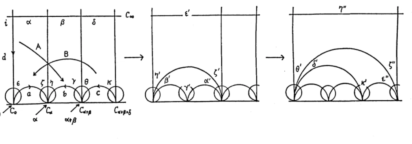
of an elementary move on $e$. The next lemma refers to Figure 4.1.

4.5. Lemma $([6,p.334])$. L-lengths

of

edges and h-lengths

of

ends

caused by the elementary move satisfy: $L_{e}L_{f}=L_{a}L_{c}+L_{b}L_{d}$,

(10)

$\alpha’=\frac{\varphi}{\varphi}\alpha=\frac{\varphi}{\epsilon}\gamma$, $\beta’=\frac{\varphi}{\epsilon}\beta=\frac{\varphi}{\varphi}\delta$,

$\gamma’=\frac{\epsilon}{\epsilon}\gamma=\frac{\epsilon}{\varphi}\alpha$, $\delta’=\frac{\epsilon}{\varphi}\delta=\frac{\epsilon}{\epsilon}\beta$.

Here and in what follows we make $\alpha$ etc., stand for the $h$-length of an

end $\alpha$ (if relevant horocycles are known) in order to simplify the notation.

For given positive numbers $\alpha,\beta,$

$\gamma$, we define a matrix

(4.6) $M(\alpha,\beta, \gamma)=-\sqrt{\frac{\gamma}{\beta}}(\begin{array}{ll}(\alpha+\beta)/\gamma \alpha 1/\gamma 1\end{array})$

.

Note that if $(a, b|c, d)=M(\alpha, \beta,\gamma)$, then

(4.7) $\alpha=b/d,$ $\beta=1/cd,$ $\gamma=d/c$.

$arrow$

Figure 4.1 The next lemma refers to Figure 4.2 which also indicates two elemen-tary moves starting on $\triangle$.

4.8. Lemma. Suppose that $L_{b}=L_{c}$ and $L_{a}=L_{d}$ hold

for

the

L-lengths. Then the linear

_{fractional transformation}

A which sends the horocycles $C_{\infty},$$C_{0}$ to $C_{\alpha+\beta},$ $C_{\alpha}$, respectively, is $M(\alpha, \beta, \gamma)$ and the linear

fractional transformation

$B$ which sends the horocycles $C_{\alpha+\beta+\delta},$ $C_{\alpha+\beta}$ to

$C_{0},$ $C_{\alpha_{J}}$ respectively, $is$

(11)

where $R$ is the linear

fractional transformation

such that _{$R(O)=\infty,$} $R(\alpha)$

$=0_{J}$ $R(\alpha+\beta)=\beta’$

,

and $\epsilon$“ is the h-length

of

the end marked by the

same letter in Figure

_4.2.

Figure 4.2 4.9. Let $S=(\alpha,$$\beta,$$\gamma,$$\delta,$ $\epsilon$, $(, \eta, \theta, \kappa)$ be the ordered set of $h$-lengths of

ends as in Figure 4.2. Then we denote by $A(S),$$B(S)$ the linear fractional transformations $A$ and $B$ in the previous lemma.

4.10. We shall establish relations between the Fricke coordinates and the $L$-length and $h$-length coordinates. Since a one-to-one

correspon-dence between the $L$-length coordinates and the $h$-length coordinates is

easily obtained by using (2.2), we need only to consider the $h$-length

co-ordinates. In what follows we consider the case

_of

$g>0$ and $s>1$

and the h-lengths

_of

ends are those with respect to horocycles

_of

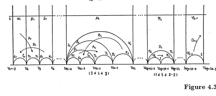
length 1. Other cases can be treated in a similar manner.

Let $D$ be the geodesic polygon constructed in 4.1. This $D$ is

trian-gulated as illustrated in Figure 4.3. Suppose that the $h$-length coordinates

are given. We shall produce the Fricke coordinates from the $h$-lengths.

For $i=1,$ $\ldots,g$, let

$S_{i}=(\alpha_{i}, \beta_{i,\gamma_{i}}, \delta_{i}, \epsilon_{i}, \zeta;, \eta_{i}, \theta_{i}, \kappa_{i})$.

Then by Lemma 4.8 we have $A_{1}=A(S_{1}),$$B_{1}=B(S_{1})$. For $i=$

$2,$

$\ldots,$$g$, consider the polygon with vertices $v_{0}(=\infty),$ $v_{4i-4},$ $v_{4i-3},$ $v_{4i-2}$,

(12)

new triangulation by vertical edges which connect $v_{0}$ and other vertices

$v_{4i-4},v_{4i-3},v_{4i-2},v_{4i-1},v_{4i}$

.

Lemma 4.5 implies that $v_{4i-4},$ $v_{4i-3},$ $v_{4i-2}$ can

be expressed in terms of the $h$-lengths in $S_{i}$ and $\lambda_{i},$

$\mu_{i},$ $\nu_{i}$. Let $R_{i}$ be

the linear fractional transformation such that $R_{i}(v_{4i-4})=\infty,$$R_{i}(v_{4i-3})=$

$0,$$R_{i}(v_{4i-2})=\alpha_{i}$. Then we have

$A_{i}=R_{i}^{-1}A(S_{i})R_{i}$, $B_{i}=R_{i}^{-1}B(S_{i})R_{i}$

.

Next consider the polygon with vertices $v_{0},$ _{$v_{4g+2i-2},$} _{$v_{4g+2i-1},$}_{$v_{4g+2i}$}, for

$i=1,$ $..,$ $s-2$

.

Operating an elementary move we obtain a

triangula-tion of this polygon by the vertical edges connecting $v_{0}$ and vertices

$v_{4g+2i-2},$ $v_{4g+2i-1},$$v_{4g+2i}(=v_{4g+2i-2}+\psi_{i})$. Then by Lemma 4.5, we can

express $v_{4g+2i-1}$ by $\sigma_{i},$ $\tau_{i},$$\varphi_{i},$$\psi_{i}$. Now the transformation $D_{i}$ is

de-termined, because $D$; fixes _{$v_{4g+2i-1}$} and sends _{$v_{4g+2i-2}$} to _{$v_{4g+2i}$}

.

Finally $D_{s-1}$ is determined by the fact that $D_{s-1}$ fixes _{$v_{4g+2s-3}$} and

sends $v_{4g+2s-4}$ to $\infty$. Thus the Fricke coordinates are determined by the

$h$-length coordinates and hence we conclude:

$v_{0}\Rightarrow\infty$

Figure 4.3 4.11. Theorem. The h-length coordinates

_defined

in 2.10 give a

global parametrization

_for

the Teichmuller space $T_{g,s}$.

(13)

[1] L.V. Ahlfors, $Lec$tures on QuasiconformalMappings, Van Nostrand, 1966

[2] A.F. Beardon, The Geometry

_of

Discrete Groups, Graduate Texts in Math. 91, Springer-Verlag, Berlin Heidelberg New York, 1983

[3] T. Nakanishi and M. N\"a\"at\"anen, The Teichm\"uller space of a punctured

surface represented as a real algebraic space, Preprint

[4] Y. Okumura, On the global real analytic coordinates for Teichm\"uller

spaces, J. Math. Soc. Japan, 42 (1990), 91-101

[5] Y. Okumura, Article in this volume

[6] R.C. Penner, The decorated Teichm\"uller _{space of punctured} surfaces,

Commun. Math. Phys. 113 (1987), 299-339

[7] P. Schmutz, Die Parametrisierung des Teichm\"ullerraumes durch

geod\"a-tische L\"angenfunktionen, Commnet. Math. Helvet. 68 (1993), 278-288 [8] M. Sepp\"al\"a and T. Sorvali, Parametrization of M\"obius groups acting in

a disk, Commnet. Math. Helvet. 61 (1986), 149-160

[9] M. Sepp\"al\"a and T. Sorvali, Parametrization of Teichm\"uller spaces by

geodesic length functions, in Holomorphic Functions and Moduli Il, (D.

Drasin et al. edt.), Mathematical Sciences Research Institute Publications 11, Springer-Verlag, Berlin Heidelberg New York, 1988, pp.267-284

[10] M. Sepp\"al\"a and T. Sorvali, Geometry