Extension of Synthesis Algorithm of Recursive Processes to
$\mu$
-calculus
$\star$
Shigetomo Kimura
(
木村成伴
),
Atsushi
Togashi
(
富樫敦
)
and
Norio
Shiratori
(
白鳥則郎
)
Research Institute
of
Electrical Communication (電気通信研究所)/Graduate Schoolof
$Inf_{\mathit{0}}r\uparrow nation$Science (情報科学研究科), Tohoku University (東北大学).
$\mathrm{e}$-mail : {kimura,togashi,$norio$
}
$@shimtori$.
riec. tohoku.$ac$.jpAbstract
In our previouswork,we proposed an inductive synthesis algorithm for recursive processes by
a subset of$\mu$-calculus. This paper presents an extension of the privious algorithm to a wide class
of$\mu$-calculus.
Keywords: Process Synthesis, Inductive Inference, Algebraic Process, CCS, $\mu$-calculus
1 Introduction
This paper proposes an extended inductive synthesis algorithm for recursive processes whichis a proper extension of the previous algorithm $[2, 3]$. To synthesize a process,
formulae of $\mu$-calculus, which must be
sat-isfiedbythetarget process,aregiventothe
algorithm one by one since such formulae exist infinitely many in general. The cor-rectnessof thealgorithm can be stated that the output sequence of processes by the al-gorithm converges to a process, which is strongly equivalent to the intended one in the limit.
Let $A$be an alphabet, a finite set of actions.
Let $C$ be a denumerable set of process con-$\overline{\star_{\mathrm{A}}}$
part of this study is supported by
Grantsfrom the Asahi Glass Foundation and
Research Funds from Japanese Ministry of
Education.
stants. Recursive terms are defined by the following BNF:
$p$ :$:=0|a.p|p+p|c$
where $c\in C$ and the meaning of $c$ is
de-fined by a defining equation $c^{\mathrm{d}}=^{\mathrm{e}\mathrm{f}}p$. A
pro-cess $c$ with the equation $c^{\mathrm{d}\mathrm{e}\mathrm{f}}=p$ is
abbrevi-ated as
rec
$c.p$.
The notions offree, bound, scope, open and closed are defined in the same way as in $\lambda$-calculus. Closed termsare called (recursive) processes. When
ev-eryfree occurrence of$c$is within some
sub-term$a.q$of$p,$ $c$is called guarded in$p$. When
every constant in $p$ is guarded, $p$ is called
guarded.
Let
72
denote the set of all processes.Se-mantics of a recursive term is given by $a$
labeled transition relation defined $\mathrm{a}\mathrm{s}arrow\subset$
$P\cross A\cross P$. For $(p, a, q)\inarrow$, we normally
write $p-^{a}q$. We use the usual
abbrevia-tions as $parrow a$ for $\exists q\in P$ such that $parrow aq$
A transition relation on recursive terms is given by the following transition rules:
$\overline{a.parrow pa}$
$\frac{parrow p’a}{p+qarrow p’a}$
(v) $p|=v\langle a\rangle f$ if there exists some $q$ such
that $p-^{a}q$ and $q\vdash-vf$
.
(vi) $p\vdash-v\mu x.f$ if $p\in S$ for all $S\subseteq P$
such that $\forall q\in \mathcal{P}.q\vdash-_{\mathcal{V}[S/x}$] $f$ implies
$q\in S$
.
$qarrow q’a$ $\underline{p\{\mathrm{r}\mathrm{e}\mathrm{c}c.p/C\}arrow paJ}$
$p+q-^{a}q’$
rec
$c.p-^{a}p’$where $p\{q/c\}$ is $p$ except any free
occur-rences of $c$ are replaced by $q$
.
A relation $R$ on $P$ is a strong bisimulation
if $(p, q)\in R$ implies, for all $a\in A$:
(i) whenever $p-^{a}p’$, then there exists $q’$
such that $q-^{a}q’$ and $(p’, q)’\in R$,
(ii) whenever $qarrow q’a$, then there exists $p’$
such that $p-^{a}p’$ and $(p’, q)’\in R$.
Recursive terms$p$and $q$are strongly
equiv-alent (written by$p\sim q$) iff $(p, q)\in R$ for
some strong bisimulation $R[5]$.
We employ $\mu$-calculus [1,4,8] to represent
properties of a process. Formulae in $\mu$
-cal-culus are defined by thefollowingBNF where
$x\in \mathcal{X}$ and $a\in A$:
$f::=\mathrm{t}\mathrm{t}|X|f\mathrm{v}f|\neg f|\langle a\rangle f|\mu x.f$
The notion of freeness,boundnessand scope
forformulae in $\mu$-calculus are defined
sim-ilarly to the one for $\lambda$-calculus. A variable
$x$ in a formula $f$is guarded, if every
occur-rence of $x$ is within some scope of $\langle a\rangle$
.
Aformula $f$ is guarded if every variable in $f$
is guarded.
Satisfactionrelation of formulae ina
valua-tion$\mathcal{V}$ (writtenby
$|=v$)is definedasfollows where $p\in P$:
(i) $p|=_{\mathcal{V}}\mathrm{t}\mathrm{t}$.
(ii) $p\models_{\mathcal{V}}x$ if$p\in \mathcal{V}(x)$
.
(iii) $p|=vf_{1}f_{2}$ if$p|=vf_{1}$ or $p|=vf_{2}$.
(iv) $p|=v\neg f$ if $p\# vf$, where $p\# vf$
means that $p$ does not satisfy $f$.
The other logical notations ff $(^{\mathrm{d}\mathrm{e}\mathrm{f}}=\neg \mathrm{t}\mathrm{t}),$
$f_{1}$A
$f_{2}(^{\mathrm{d}\mathrm{e}i}=\neg(\neg fi\vee\neg f_{2})),$ $[a]f(^{\mathrm{d}}=^{\mathrm{e}t}\neg\langle a\rangle\neg f)$, and
$\mathcal{U}X.f(X)(^{\mathrm{d}}=^{\mathrm{e}\mathrm{f}}\neg\mu x.\neg f(\neg x))$can bedefined as
usual.
Proposition 1 [1] Let$f(x)$ be a guarded
formula, then we have:
(i) $\mu x.f(_{X})\equiv _{k>0f^{k}()}\mathrm{f}\mathrm{f}$
.
(ii) $\nu x.f(x)\equiv\wedge k>0fk(\mathrm{t}\mathrm{t})$. $\square$
Proposition 2 [1] Processes$p$ and $q$ are
strongly equivalent, $i.e$. $p\sim q$,
iff
$\mathcal{L}(p)=$$L(q)$ where $\mathcal{L}$ is the set
of
all closed$f_{orm}u_{\square }-$$lae$ and $\mathcal{L}(p)\mathrm{d}=\mathrm{e}\mathrm{f}\{f\in \mathcal{L}|p|=f\}$
.
In thefollowing,aformula,which expresses necessary and sufficientproperties of a pro-cess, is defined. Let $C$ be a set of process
constants. $F_{C}$ : $Parrow \mathcal{L}$ is a function
de-fined in the followingway:
(i) $F_{C}(0)=\wedge a\in A[a]\mathrm{f}\mathrm{f}$.
(ii) $Fc(a.p)$
$=\langle a\rangle Fc(p)$A$[a]F_{C}(p)\Lambda\wedge b\in A-\{a\}[b]\mathrm{f}\mathrm{f}$
.
(iii) $F_{C}(a_{1\cdot p1}+\cdots+a_{n}.p_{n})$
$=( \bigwedge_{i\in I}\langle a_{i}\rangle \mathcal{F}_{C}^{\cdot}(p_{i}))$ A $(\wedge i\in I[a_{i}]\mathrm{v}a_{i}=a_{j}c\mathcal{F}(p_{j}))$
A $( \bigwedge_{a\in AA}-[a]\mathrm{f}\mathrm{f})$ where $n\geq 2,$ $I=$
$\{1, \ldots,n\}$ and $A=\{a_{i}|i\in I$ and
$a_{i}\in A\}$.
(iv) $F_{C}(C)=\{$
$\nu x_{\mathrm{c}}.F_{C\cup\{_{\mathrm{C}}\}}(p)$ if$c\not\in C$
$x_{c}$ if $c\in C$
where$x_{c}$ is a fresh variable and $c^{\mathrm{d}}=^{\mathrm{e}\mathrm{f}}p$
.
Proposition 3 $[1, 3]$ Let$p$ and $q$ be
pro-cesses:
(ii) $p\sim q$
iff
$q\vdash-F_{\phi}(p)$.
$\square$Proposition 4 [7] Any
formula
can beequivalently converted to a
formula
with-out negation, $i.e$.
aformula
built$upwith\square$ $\mathrm{t}\mathrm{t}_{r}\mathrm{f}\mathrm{f}_{y}\wedge,$ $,$ $\langle$$a)$, $[a],$
$\mu$, and $\nu$
.
From now on, we will consider closed for-mulae without negation.
2 Synthesis algorithm
A synthesis algorithm proposed here is an inductive one. It generates a process which
satisfies given facts or properties of the in-tended target process. These facts are rep-resented as formulae in $\mu$-calculus and the
inputtothe algorithm is an enumeration of formulae to be satisfied by the target pro-cess. Let$p_{\mathit{0}}$ be the intended target process.
It should be noted that $p_{\mathit{0}}$isneither known
initially nor given in a precise manner.
Definition 5 Let $U$ be a set
of
pairsof
’
formulae
$f\in \mathcal{L}$ and $signs+_{f}$ -, $i.e$
.
$\langle f, +\rangle$(or$\langle f,$$-\rangle$) such that either$\langle f, +\rangle$ or$\langle f, -\rangle$
always belongs to $U$
for
everyformula
$f\in$L. $S=\{f|\langle f, +\rangle\in U\}\cup\{\neg f|\langle f, -\rangle\in$
$U\}$ is an enumerationof facts
if
$S$ iscon-sistent in the deductive system $STL(\mathcal{X}, A)$
[1]. An element
of
$S$ is called $a$fact. $\square$Given an enumeration of facts, the
algo-rithm synthesizes a process satisfying those facts. A process can be represented as a
term $p$ with a set $\{c_{1}\mathrm{d}\mathrm{e}t=p1, \ldots, c_{n}\mathrm{d}\mathrm{e}=^{\mathrm{f}}p_{n}\}$
of defining equations. In the algorithm, a process is represented as an identified
pro-cess constant with a set of process
defini-tions. Each process definition
rec
$c.p$ isas-sociated with aset $C$ of formulae, denoted
as $c:C$, which must be satisfied by the
cor-responding process constant $c$
.
$C$ can be$o$mitted when it is not important.
In $[2, 3]$, we proposed the synthesis
algo-rithmwhich constructed recursiveprocesses by formulae in $\mu$-calculus without $\neg,$ ${ }$ nor
$\mu$ operator. Formulae with ${ }$ operator are
ambiguous to synthesize processes. Espe-cially,since aformulawith $\mu$ operator (a$\mu-$
formula for short) involves infinitely many
${ }$operators (see Proposition 1), it may cause
backtracking infinite many times.
From this restriction, the limit process of the output sequence of the algorithm may not be equivalente to the intended target one. In fact, the limit process satisfies more properties than the target process. So, the
formulae including V or $\mu$ operators show
that an output process of the algorithm satisfies $\mathrm{s}o$me undesirable propeties. To
complete the synthesis algorithm, the
re-striction for the input formulae must be relaxed.
The algorithm in Fig. 1 is an extension of the one in $[2, 3]$. This algorithm admits
to input formulae involving $\mu$ or ${ }$
oper-ators. Unfortunately, the following restric-tions remain. First, any $\mu$ or $\nu$ operators
must not occurr within the scope of the
$\mu$ operator. Second, any $\mu$ operators must
not occurrwithin the scope of the $\nu$
opera-tor. Todescribe the algorithm, we adopt a language like Prolog, where $\mathrm{I}/\mathrm{O}$ predicates
can backtrack as well. For brief descrip-tion, let $c_{i}$ denote process constants
asso-ciating with the process definitions $c_{i}=p_{i}\mathrm{d}\mathrm{e}i$
or $c_{i}:C_{i}\mathrm{d}=pi\mathrm{e}\mathrm{t}$ where $C_{i}$ is a set of formulae.
The initial state of a process is always fixed
to $c_{0}$. Thus, a set
$\{c_{0^{\mathrm{d}}=}p\mathrm{o}, \ldots, c_{n}=^{\mathrm{e}}pn\}\mathrm{e}\mathrm{f}\mathrm{d}t$of
$\mathrm{p}\mathrm{r}o$cess definitions determines the process
$c_{0}$ with its set of process definitions. In the
algorithm, the
following
abbreviations areadopted:
A
$\{f_{1}, \ldots, f_{n}\}=f_{1}$ A...
A$f_{n}$ where $\wedge\emptyset^{\mathrm{d}}=^{\mathrm{e}i}$ $\mathrm{t}\mathrm{t}$.
$S[c_{1}:c_{1}\mathrm{d}\mathrm{e}t=p_{1}, \cdots, c_{k}:C_{k}\mathrm{d}\mathrm{e}\mathrm{f}=p_{k}]$
:
Thethe process definitions of$c_{1},$ $\cdots,$$c_{k}$ in $S$ fication color. When the algorithm makes
are replaced by $c_{1}:C_{1}\mathrm{d}\iota=^{\mathrm{e}}p_{1},$ $\cdots,C_{k}:C_{k}\mathrm{d}=\mathrm{e}\mathrm{f}$ branches in a process
graph, i.e. an
ac-$p_{k}$,respectively, or $c_{i}:C_{i}\mathrm{d}\mathrm{e}ip=i$ is addedto tion prefix of the process, or traces
them
$S$ if$c_{i}:c_{i}\mathrm{d}=p_{i}\mathrm{e}i\not\in S$. by
$\langle a\rangle$ or $[a]$ oparetors, the formula draws
$S\{x/y\}$ : The resulting $S$ where a free a line with its own color beside them. In
variable $y$ is substituted for $x$ in S. the former case, solid lines areused. In the
latter case, dashed lines are used. Using
Algorithm 1 (Synthesis algorithm) colored lines, the algorithm finds whether
or not backtracking procedure occurs in-Input: Enumeration
of
facts
$f_{1},f_{2_{f}}\cdots$.
Itfinitely manytimes. Suppose aformula$\mu x$
.
is an enumeration
of formulae
be satis- $f(x)$ is input to the algorithm. Thealgo-fied
by the intended target process. The rithm traces a current process or makesorder
of
them is arbitrary. new branches to construct a processsatis-Output: Sequence
of inferred
processes$p_{1_{l}}$fying the input formula. If the traced path
$p_{2;}\cdots$
.
Each $p_{k}$satisfies
the whole inputhas no loops, $f(x)$ cannot be satisfied
in-formulae
$f_{1}$ to $f_{k}$.
finitely many times. More precisely, it can
Predicates: See Fig. 1. $\square$
be the case that $f(x)$ is built up only with In the following, the extended parts of the $\langle a\rangle,$ ${ }$ and A operators, e.g. $\langle a\rangle\langle b\rangle_{X}$. But
$\mu x.\langle a\rangle\langle b\rangle X$ is logically equivalent to ff. So
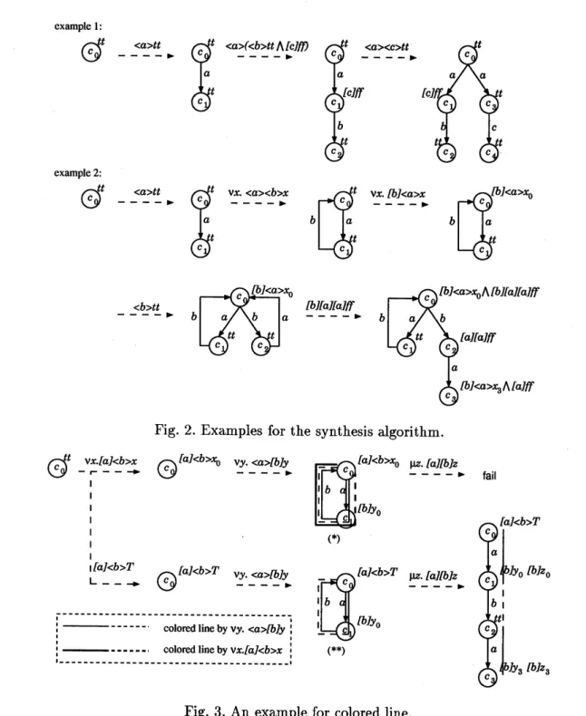
algorithm from [2] will be explained. For
suchformulaearereduced to ff when these
the partsof[2],examples are given in Fig.2
formulaeare input (by
remove-consistent-One of the extensions is for the operator $mu$ of$mp(S)$ inAlgorithm 1). If the traced
${ }$ in (g).
One
of the subformula of V is path has loops but each loop is not fullyapplied first to the current process, and if it (notpartially) drawnby colored solid lines, happens to be inconsistent to the process, then$f(x)$ cannotbe satisfied infinitely. But the other subformulais applied. there is a path drawn fully, then $f(x)$ may be satisfiable. See Fig.3 and4 as examples. The other extension is for $\mu$-forumlae in In Fig.3, each process
$(^{*})$ and $(^{**})$ has a
(c). Theformula$\mu x.f(x)$ says that the tar- loop satisfying $[a][b]_{Z}$ infinitely. The loop get process satisfies $f(x)$ repeatedly finite of $(^{*})$ is fully drawnby a colored solid line
times, but must not execute infinite many (for$a$-branchby a thin line and $b$by a thick
times. When $\mu x.f(x)$ is input to the syn- line). So $\mu z.[\mathit{0}][b]z$ is inconsistent to the
thesis algorithm, it checks that whether or process $(^{*})$. On the other hand, the $(^{**})’ \mathrm{s}$
not the current process satisfies $f(x)$ in- loop is not fully drawn, i.e. b–branch is not finitely many times, i.e. whether or not the drawnbysolidline. Thus $(^{**})$ is
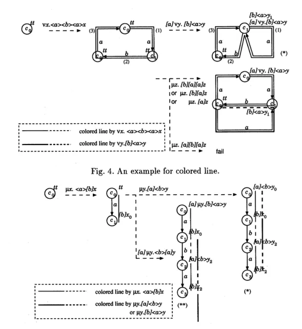
backtrack-process has loops satisfying $f(x)$ infinitely. able. However any fully drawn loop does Ifit does, the algorithm backtracks to the not occur inconsistent. In Fig.4, the pro-point before one of such loops was made. cess $(^{*})$ has the fully drawn loop. But for-But even after backtracking, the synthe- mulae $\mu z.[b][a][\mathit{0}]_{\mathcal{Z}},$ $\mu z.[b][a]Z$ and $\mu z.[a]z$
sized process may satisfy theformula $f(x)$ does not occur inconsistent, since the or-infinitely. In such cases, the backtracking der of the traced path by each formula dif-will occur infinitely, so the synthesis al- fers from the one ofcolored line. Therefore gorithm never terminates. The basic idea the algorithm must also check whether or
fortermination is to check theexistence of not the orders of them are identified. This
such fatal loops by drawing colored lines. is why the dashed lines are needed. Some
in-mpstart:-$mp\langle\{c_{0}:\{\mathrm{t}\mathrm{t}\}=^{t}0\mathrm{d}\mathrm{e}\})$. makeproc-mu$(\mathrm{C}\dot{\iota}, s, xg’ \mathrm{X})$ :-% Where$i\neq j$.
% The initial processis$0$. no-colored-cycle,
$mp(S)$ :-% $S$isa set ofprocessdefinitions. no-overlappe$d- mu- pa\iota h$,
read-formula$(!)$, $mak\mathrm{e}proC\mathrm{t}c_{1},$$S,$$f(x_{\mathrm{J}}),\mathrm{X})$. $\ldots\ldots\ldots\ldots\ldots\ldots\ldots\ldots..(\mathrm{c}^{*})$ % lnputa formula. % $\langle a\rangle f\ldots\ldots\ldots\ldots\ldots\ldots\ldots\ldots\ldots\ldots\ldots\ldots\ldots\ldots\ldots\ldots(\mathrm{d})$
$conver\iota-formula(f, f’)$, makeproc($\mathrm{C}:,$$S,$$(a\rangle j,\mathrm{X})$ :-% $\mu x(1a$]$x\wedge(a\rangle$$(b\rangle\iota\iota)$ transii
$(cj, a, C:)$, % $\exists c_{j}$ suchthat$\mathrm{c}:arrow c_{j}a$.
% $-arrow\mu x$.$(1a]_{X}\wedge(a)(x\wedge(b\rangle\iota \mathrm{t})) fre\mathrm{e}-variables1f,\mathrm{c})$,
% $\nu x([a]1b1^{x}$A($a\rangle\langle b\rangle(c\rangle \mathrm{t}t)$
% get freevariablesof$f$toC.
% $-arrow\nu x.([a]1b1^{x}\wedge(a\rangle([b]x\wedge(b\rangle 1x\wedge\langle c\rangle t\iota)))$ $full- C\circ l_{\mathit{0}}ring$(
$a,$ci,$\mathrm{C},\mathrm{C}$)
$j$ ’
$remove- Consi_{St}\mathrm{e}nt-mu(j’, j’’)$, %drawlines colored by every color of$\mathrm{C}$
% $1\mathrm{f}$asubfomulaof$j’$isof a$\mathrm{f}\mathrm{o}\mathrm{m}\mu x.g$and$g$ %beside the
$a$-branch from$c_{1}$ to$c_{j}$ %has $\langle a\rangle,$${ }$and$\wedge$operators andvariable$x$ makeproc$(\mathrm{c}_{j}, S, !,\mathrm{X})$.
%but not others, then$\mu x.g$ismodified by$\mathrm{f}\mathrm{f}$.
makeproc$(\mathrm{C}:, S, (a)j,\mathrm{X})$
:-% e.g. $1a1\mu x.(a\rangle(b\rangle Xrightarrow[a]R.$ $g\mathrm{e}\iota_{- n\mathrm{e}wr\mathit{0}c}-peSS- constant(c_{J})$,
makeproc$(c_{0}, s, f’’,\mathrm{X})$, jree-variables
$(j,\mathrm{c})$,
% Modify the current process according to $full- \mathrm{c}olor:ng(a, C:, cj,\mathrm{C})$,
%thenewfact$j”$, the resultissettoX.
makeproc$(\mathrm{C}j,$$s[c|c:|\mathrm{d}\mathrm{e}\mathrm{I}=p_{1}+a.c_{j}, c_{j}:\{\mathrm{t}\mathrm{t}\}\mathrm{d}\mathrm{e}t=0]$,
$write- pro\mathrm{C}\mathrm{e}ss(\mathrm{x})$, % Output the result.
$f\wedge(\wedge\{fk|[a]j_{k}\in C:\}\rangle,\mathrm{x})$. .. . . .... . . ... .... ...$(\mathrm{d}^{*})$
$mp(\mathrm{X})$.
% $[a]f\ldots\ldots\ldots\ldots\ldots\ldots\ldots\ldots\ldots\ldots\ldots\ldots\ldots\ldots\ldots\ldots.(\mathrm{e})$
% Continuethe synthesis for the next fact.
% program clausesof makeproc$(\mathrm{c}, S, f,\mathrm{X})$ makeproc
$(c_{i}, s, [a]f, s)$
:-% $c$: the current process constant
$i_{S- v}a\iota id(\wedge C_{1}\supset[a]j)$. $\%\models\wedge C_{\dot{\iota}}\supset[a]f$
% $S$: the current set of processdefimitions makeproc$(c:, S, [a]f, S1^{c:}:(c_{:\cup}\{[a]j\})\mathrm{d}\mathrm{e}\mathrm{f}=pi]):-$ % $f$: thecurrentformulato besatisfiedby$\mathrm{c}$ $not-tranSit(\mathrm{c}_{1}., a).$% $c_{i}\neq t$.
% $\mathrm{X}:$infeITed process($\mathrm{S}\mathrm{e}\iota$ofprocessdeffiuitions) makeproc(
$c_{\mathfrak{i}},$$S,$$[a]j,\mathrm{x}_{)}$
:-%Note $c,S,f$are meta variables. $jr\mathrm{e}\mathrm{e}- variab\iota \mathrm{e}s(f,\mathrm{C})$,
$broken-\iota in\mathrm{e}- \mathrm{C}o\iota oring(a, \mathrm{c}:, \mathrm{c}j,\mathrm{C})$,
% $\mathrm{t}\mathrm{t}\ldots\ldots\ldots\ldots\ldots\ldots\ldots\ldots\ldots\ldots\ldots\ldots\ldots\ldots\ldots\ldots..(\mathrm{a})$ % draw dashedlinescoloredby every colorof$\mathrm{C}$
makeproc$(\mathrm{c}i, S,\iota\iota, S)$ % beside the
$a$-branchfor all$c_{j}.c:arrow a\mathrm{c}_{j}$.
% $x_{j}$ :abound variable corresponding to the
$fora\iota\iota\langle \mathrm{c}_{\mathrm{J}},$$c:,$$s[\mathrm{C}::C_{i}\cup\{[a]f\}=\mathrm{d}\mathrm{e}\mathrm{I}p:],$$f,\mathrm{x})$. %fomula$\nu x_{j}.f(x_{\mathcal{J}})\ldots\ldots,$$\ldots\ldots\ldots\ldots\ldots\ldots\ldots\ldots\ldots(\mathrm{b})$
$mak\mathrm{e}pro\mathrm{C}\langle_{\mathrm{C}}:,$$S,$$x_{j},\mathrm{X}$)$.-$ %
$\forall \mathrm{c}_{j}.\mathrm{c}_{i}arrow c_{j}a$,
$is- nu$-variable$\mathrm{t}Xj$),
makeproc$(Cj, s[c_{\dot{*}}:C\dot{2}\cup\{[a1^{j\}=pi}\mathrm{d}\mathrm{e}\mathrm{r}], f,\mathrm{X})$.
% $1\mathrm{s}x_{j}$ avariable of a$\nu- \mathrm{f}\mathrm{o}\mathrm{m}\mathrm{u}\mathrm{l}\mathrm{a}$?
% $f_{1}\wedge j_{2}\ldots\ldots\ldots\ldots\ldots\ldots\ldots\ldots\ldots\ldots\ldots\ldots\ldots\ldots\ldots.(\mathrm{f})$
$mak\mathrm{e}proc-nu(\mathrm{Q}, s_{x_{j},\mathrm{x})},. makeproc1^{c,S}i, !1\wedge f_{2},\mathrm{X})$
:-$makepro\mathrm{C}-nu(\mathrm{C}i, s, X_{l}, S)$. makeproc$(c_{i}, S, f_{1},\mathrm{Y})$,
$makeproc- nu\mathrm{t}c:,$$S,$$xj,\mathrm{X})$ :- %Where$i\neq j$. makeproc
$(c:,\mathrm{Y}, f2,\mathrm{X})$.
$S’arrow(S[c_{j}:C_{j}\mathrm{d}\epsilon=^{q}p:+p_{j}]-$ % $f_{1}\vee f_{2}\ldots\ldots\ldots\ldots\ldots\ldots\ldots\ldots\ldots\ldots\ldots\ldots\ldots\ldots\ldots(\mathrm{g})$
$\{\mathrm{c}_{i}:C_{i}\mathrm{d}\epsilon \mathrm{I}=p:\})\{xj/X:\}\{c_{j}/c_{i}\}$, makeproc$(c:, S, j1f_{2},\mathrm{X})$
:-makeproc$(\mathrm{C}i, s, f1,\mathrm{x})$.
makeprocl$cj,$$S’,$$\wedge c_{i},\mathrm{X}$). .. . . .... .. ... ... . . .. .$(\mathrm{b}^{*})$
$mak_{6}proc(c_{i}, s, f_{1}\vee j_{2},\mathrm{X})$
:-mak$\mathrm{e}\mathrm{p}roc-nu\mathrm{t}c_{1},$$S,$$x_{j},\mathrm{x}$)
:-makeproc$(c,, S, j2,\mathrm{X})$.
is-remake, %canbacktrack?
makeproc$(\mathrm{C},, S, !\mathrm{t}Xj\rangle,\mathrm{x})$. . .. . . .. .. .. .... ..
.
.$(\mathrm{b}^{**})$ %$\nu x.f(x)\ldots\ldots\ldots\ldots\ldots\ldots\ldots\ldots\ldots\ldots\ldots\ldots\ldots\ldots\ldots\langle \mathrm{h})$
makeproc$(C_{1}, s, \nu x.f(x),\mathrm{X})$
:-% $x_{j}$ : a boundvariable corresponding to the
$get-fr\mathrm{e}sh_{\mathrm{C}}- \mathit{0}\iota or(\mathrm{C})$,
%formula$\mu_{X_{j}}.!1x_{j}$) $\ldots\ldots\ldots\ldots\ldots\ldots\ldots\ldots\ldots\ldots\ldots.\langle \mathrm{c})$
makeproc$(C_{\dot{l}}, S,x_{j},\mathrm{x})$
:-$\mathrm{c}o\iota_{or}ing- t_{\mathit{0}-}variabl\mathrm{e}(x,\mathrm{c})$, $makepro\mathrm{c}\langle_{\mathrm{C}}i,$$s,$$f\mathrm{t}x_{\dot{*}}),\mathrm{X})$.
$i_{S-m}u-variab\iota_{\mathrm{e}\mathrm{t})}Xj$,
% $\mu x.f(x)\ldots\ldots\ldots\ldots\ldots\ldots\ldots\ldots\ldots\ldots\ldots\ldots\ldots\ldots\ldots(\mathrm{i})$
% ls$x_{j}$ avariableof a$\mu- \mathrm{f}\mathrm{o}\mathrm{m}\mathrm{u}\mathrm{l}\mathrm{a}^{?}$
makeproc$(c_{1}, S,\mu x.f\mathrm{t}X),\mathrm{x})$ :-$mak\mathrm{e}pro\mathrm{c}-mu(\mathrm{c}:, S, x_{j},\mathrm{X})$.
$makepro\mathrm{C}-mu(\mathrm{c}_{i},$$s,$$x|’ \mathrm{X}\rangle$ $.-$fail.
$g\mathrm{e}t- fr\mathrm{e}sh-Color(\mathrm{c})$,
$coloring-t\not\in variab\iota 6(X,\mathrm{c})$,
makeproc$(c:, S, f\langle x_{i}),\mathrm{X})$.
Fig. 1. The synthesis algorithm
finite branches. See Fig.5. $\ln$ such cases,
each colored line by $\mu$-formulae are
over-lapped, and if one $\mu$-formula draws a solid
line, the others draw dashed lines. In the rest of paper, these pairs of lines are called overlapped $\mu$-paths. In Fig.5, the $\mathrm{P}^{\mathrm{T}\mathrm{o}\mathrm{C}\mathrm{e}\mathrm{S}\mathrm{s}}$ $(^{*})$ has overlapped $\mu$-paths. Each a-branch
is drawn by thin solid lineand thickdashed
line. And the b–branch is drawn by reverse
order of the above. The process $(^{**})$ is the
same case, though starting points of each lines are difference.
Theorem 6 Assume thatthere exists a pro-cess satisfying initial segments $f_{1},$
$\cdots,$$f_{n}$
of
an enumerationof
facts, where $n\geq 1$.
Assume Algo$7^{\cdot}ithm\mathit{1}$ outputs a set
of
example1:
$G^{c}t$ $—-<a>tt>$
example2:
$\Theta^{tt}c$ $—-<a>tt$
.
$\mathrm{V}X.<a><---b>x$$–<\underline{b}>\underline{tt}$
.
$\mathrm{v}x\underline{l}bJ<a>x-\cdot-\cdot$
$\underline{Ib}\underline{Jf}a]Ia]--ff$
Fig. 2. Examples for the synthesis algorithm.
$G^{c}t-\ulcorner \mathrm{v}x.\mathrm{f}a]-<b->xarrow$ $\Theta^{c}fa]<b>x0$ $\mathrm{v}y<a>l-\cdot----b]y$
tail 1 1 1 1 $1$ 1 $\llcorner \mathrm{l}fa|-J<b>T-arrow$
\copyright
$faJ\tau<b>$ $\mathrm{v}y.<a--->lb]y$ $1—————————————|$ $1$ coloredline by$\mathrm{v}y$.$<a>[b\mathit{1}_{\mathcal{Y}}\mathrm{I}|$$1$
$11——-$
coloredline by$\mathrm{v}x.faJ<b>X11$$1_{----}1---|1$
Fig. 3. An example for colored line.
$f_{1},$
$\cdots,$$f_{n-1}$ also. For the n-th fact, $f_{n_{f}}$ the
followings are
satisfied:
(i) The algorithm terminates and outputs a set
of
processdefinitions
$S_{n}$ with theprocess constant$c_{0}$ (the initial state
of
$S_{n})$.
(ii) $c_{0}$ with $S_{n}$
satisfies
$f_{n}$.
(iii) $c_{0}$ with $S_{n}$
satisfies
$f_{1},$$,$$..,$$f_{n-1}$.
Proof.[sketchofproof] (i) When the pred-icate makeproc callsitself recursively, let $f$
be a givenformulatoit, and $g$ be aformula
to call itself. Then, the size of$g-$the
num-ber of operators constructing the formula
–can be greater than the size of $f$, only
in the clauses $(\mathrm{b}^{*}),$ $(\mathrm{b}^{**}),$ $(\mathrm{c}^{*})$ and $(\mathrm{d}^{*})$
in Algorithm 1. Without using the above
There-$G^{c}t$
Fig. 4. An example for colored line.
Fig. 5. An examplefor overlapped $\mu$-paths
fore, it is sufficient to consider them only. Suppose the algorithm dose not terminate for some input formulae. Then the follow-ing seven cases must be considered.
(1) $(\mathrm{b}^{*})$ and $(\mathrm{b}^{**})$ occur infinitely, but none
of other cases do.
(2) $(\mathrm{c}^{*})$ does, but none of other cases do.
(3) $(\mathrm{d}^{*})$ does, but none of other cases do.
(4) $(\mathrm{b}^{*}),(\mathrm{b}^{**})$ and $(\mathrm{c}^{*})$ do, but $(\mathrm{d}^{*})$ does
not.
(5) $(\mathrm{b}^{*}),(\mathrm{b}^{**})$ and $(\mathrm{d}^{*})$ do, but $(\mathrm{c}^{*})$ does
not.
(6) $(\mathrm{c}^{*})$ and $(\mathrm{d}^{*})$ do, but not $(\mathrm{b}^{*})$ and $(\mathrm{b}^{**})$
.
(7) The whole cases do.
The impossibility ofcases (1), (2) and (4) is already proved in [3]. The one of other
casesischecked by the following predicates.
(3) by$convert- f_{\mathit{0}}rmula(f, f’)$and
remove-$conS\dot{i}stent- mu(f’, f’’)$ in $mp(S)$
.
(5) by no-overlapped-mu-path in $(\mathrm{c}^{*})$
.
(6) by $no- colored- Cy_{C}le$ in $(\mathrm{c}^{*})$.
(7) by no-colored-cycle in $(\mathrm{c}^{*})$and
remove-consistent-mu$(f’, f”)$ in $mp(S)$.
(ii) and (iii) The proof of them are almost
The algorithm is a non terminating
pro-cedure. Therefore, we show its correctness
byusing the concept ofconvergencein the
limit, which has been a key idea in
induc-tivelearning paradigm [6].
Definition
7
Assume an algorithm readsin an enumeration
of
facts, and returnsprocesses sequentially.
After
some time,if
the output process is always$p$, then the
in-ferred
sequence by this algorithm converges in the limit to $p$ over the enumerationof
facts.
$\square$Lemma 8 Assume $p$ is an intended
pro-cess, andthe
inferred
sequenceof
processes by the Algorithm 1 converges in the limit to a process$p’$. Then $p\sim p’$. $\square$The validity of Algorithm 1 is also shown
by thefollowing theorem.
Theorem 9 Under the assumption
of
al-gorithm 1,
if
there exists a process$p$satis-fying an enumeration
of
$factS_{f}$ theinferred
sequence
of
processes by Algorithm 1con-verges in the limit to a process$p’$ such that
$p\sim p’$.
Proof. By Proposition 3, Theorem 6 and
Lemma 8. $\square$
References
[1] Graf, S. and J. Sifakis: “A Logic for
the Description of Non-deterministic Programs and Their Properties”, Inf. and contr., 68, $\mathrm{p}\mathrm{p}.254^{-27}0(1986)$
[2] Kimura,S., A. Togashi and N. Shiratori: “Synthesis Algorithm for Recursive
Processes by $\mu$-calculus”, Lecture Notes
in Artificial InteUigence, 872,
pp.379-394(1994)
[3] Kimura, S., A. Togashi and N. Shiratori:
“Inductive
Synthesis of Recursive Processes from
Logical Properties”, Information and
Computation, (submitted)
[4] Kozen,D.: “Resultson thePropositional
$\mu$-calculus”, Theoret. Comput. Sci., 27,
$\mathrm{p}\mathrm{p}.333^{-}354(1983)$.
[5] Milner, R.: “Communication and
Concurrency”, Prentice-Ha11(1989).
[6] Shapiro, E.Y.: “Inductive Inference of
Theories From Facts”, Technical Report
192, Yale Univ(1981).
[7] Stirling,
C.: “Modal Logics For Communicating
Systems”, Theoretical Computer
Science, 49,$\mathrm{P}\mathrm{P}^{311-34}.7(1987)$
.
[8] Stirling, C.: “An Introduction to Modal
and Temporal Logics for CCS”, Lecture
Notes in Comput. Sci. 491,
Springer-Verlag,$\mathrm{p}\mathrm{p}.2-20(1991)$
.
3
Conclusion
Thispaper presents the synthesis algorithm,
whichis extention of the algorithmin [2,3],
for a recursive process. We show the out-put sequence of the algorithm converses to a process which is strong equivalent to the target one in the limit.
[9]Togashi, A. and S. Kimura: “Inductive
Inference of Algebraic Processes based on
Hennessy-Milner Logic”, Trans. IEICE,