トップ - アジア経済研究所学術研究リポジトリ ARRIDE

Export platform foreign direct investment :

theory and evidence

著者

Ito Tadashi

権利

Copyrights 日本貿易振興機構（ジェトロ）アジア

経済研究所 / Institute of Developing

Economies, Japan External Trade Organization

(IDE-JETRO) http://www.ide.go.jp

journal or

publication title

IDE Discussion Paper

volume

378

year

2012-12-01

INSTITUTE OF DEVELOPING ECONOMIES

IDE Discussion Papers are preliminary materials circulated to stimulate discussions and critical comments

Keywords: Export platform FDI JEL classification: F12, F15, F23

* Inter-Disciplinary Studies Center, IDE (Tadashi_Ito at ide.go.jp)

IDE DISCUSSION PAPER No. 378

Export Platform Foreign Direct

Investment: Theory and Evidence

Tadashi ITO

*

December 2012

Abstract

This paper proposes a model that accounts for “export platform” FDI – a form of FDI that is common in the data but rarely discussed in the theoretical literature. Unlike the previous literature, this paper’s theory nests all the typical modes of supply, including exports, horizontal and vertical FDI, horizontal and vertical export platform FDI. The theory yields the testable hypothesis that a decrease in either inter-regional or intra-regional trade costs induces firms to choose export platform FDI. The empirical analysis provides descriptive statistics which point to large proportions of third country exports of US FDI, and an econometric analysis, whose results are in line with the model’s predictions. The last section suggests policy implications for nations seeking to attract FDI.

The Institute of Developing Economies (IDE) is a semigovernmental, nonpartisan, nonprofit research institute, founded in 1958. The Institute merged with the Japan External Trade Organization (JETRO) on July 1, 1998. The Institute conducts basic and comprehensive studies on economic and related affairs in all developing countries and regions, including Asia, the Middle East, Africa, Latin America, Oceania, and Eastern Europe.

The views expressed in this publication are those of the author(s). Publication does not imply endorsement by the Institute of Developing Economies of any of the views expressed within.

INSTITUTE OF DEVELOPING ECONOMIES (IDE), JETRO 3-2-2, WAKABA,MIHAMA-KU,CHIBA-SHI

CHIBA 261-8545, JAPAN

©2012 by Institute of Developing Economies, JETRO

No part of this publication may be reproduced without the prior permission of the IDE-JETRO.

Export Platform Foreign Direct Investment: Theory and

Evidence

Tadashi Ito¨

Institute of Developing Economies, Japan

October 2012

Abstract:

This paper proposes a model that accounts for “export platform” FDI – a form of FDI that is common in the data but rarely discussed in the theoretical literature. Unlike the previous literature, this paper’s theory nests all the typical modes of supply, including exports, horizontal and vertical FDI, horizontal and vertical export platform FDI. The theory yields the testable hypothesis that a decrease in either inter-regional or intra-regional trade costs induces firms to choose export platform FDI. The empirical analysis provides descriptive statistics which point to large proportions of third country exports of US FDI, and an econometric analysis, whose results are in line with the model’s predictions. The last section suggests policy implications for nations seeking to attract FDI.

Key words: Export platform FDI JEL Classification: F12, F15, F23

* IDE-JETRO, 3-2-2 Wakaba, Mihama-ku, Chiba-shi, Chiba, 261-8545, Japan;

[email protected], or [email protected]. I am grateful to my thesis adviser, Professor Richard E. Baldwin at the Graduate Institute, Geneva for his invaluable advice. I would also like to express my sincere gratitude to anonymous referee(s) and the editor of this journal for their invaluable suggestions and to the seminar participants at ETSG 2010, Keio University, and Chukyo University for their useful comments.

1. I

NTRODUCTION

The complexity of modes of foreign direct investment (FDI) has recently been discussed in the literature. The old framework of horizontal and vertical FDI does not represent well the actual modes of FDI. Firms set up plants not only to supply the host country’s market but also the host nation’s neighbouring countries. For example, many tobacco companies have their European headquarters and plants in Switzerland. The world’s largest Vinyl Chrolide Mononer1 producer, Shinetsu Chemical has its plants in Portugal and supplies all European countries from there. In Far East Asia, parts and components are produced and shipped back and forth among many countries in the region2 before they are sold as final products.

To see if export platform type FDI is an important phenomenon, we have computed the ratio of exports to third countries over the total sales of US FDI3 (Figure 1). We have taken the top 20 countries with the largest US FDI stock in 2008, the most recent year for which data are available. Countries are ordered by the US FDI stock amount. The United Kingdom is the largest recipient of US FDI, followed by the Netherlands. We notice that small countries, such as the Netherlands, Luxembourg, Ireland, Switzerland, Belgium, Singapore and Hong Kong have high ratios of exports to third countries, ranging from about 40 to 70 percent. Large EU countries, such as the United Kingdom, France, Germany and Spain exhibit 20 to 30 percent. On the other hand, also large but non-EU countries, which do not have neighbouring countries of similar income level, such as China and Japan show rather small numbers. These findings imply export platform FDI is prevalent in countries (especially small countries) which have neighbouring countries of similar income level and also that the EU might have induced export platform type FDI by reducing intra-regional trade costs within EU countries.

1 A basic raw material for plastics used mainly for construction

This paper constructs a model with export platform FDI. Unlike previous theoretical work it attempts to nest all types of FDI in one model. The model shows that a reduction in trade costs, either inter-regional and/or intra-regional, induces firms to choose export platform FDI rather than other modes of supply. The empirical part of the paper corroborates this theoretical prediction, using US outward FDI.

Figure 1: Third country export ratios of the top 20 US FDI recipient countries

0.0% 10.0% 20.0% 30.0% 40.0% 50.0% 60.0% 70.0% 80.0% U n it e d K in g d o m N e th e rl a n d s C a n a d a L u x e m b o u rg B e rm u d a Ir e la n d Ge rm a n y Ja p a n S w it z e rla n d F ra n c e B e lg iu m A u st ra lia S in g a p o re M e x ico It a ly S p a in C h in a B ra z il H o n g K o n g Ko re a

Source: Author’s computation from the data of Bureau of Economic Analysis (BEA)

Literature

Many economists argue that the modes of supply of multinational firms are more complex than the pioneering works of horizontal and vertical FDI by Helpman and Krugman (1985). Unlike the usual model of FDI (Markusen (2002)), in which horizontal FDI is a substitute for trade, Bergstrand and Egger (2007) develop a model where horizontal FDI coexists with trade between identical countries. Yeaple (2003) constructs a model where a firm may engage both in horizontal and vertical FDI, for a medium range of trade costs.

The literature on export-platform FDI is surveyed by Greenaway and Kneller (2007). As it appears in this survey paper, Motta and Norman (1996) is probably the first paper to theoretically deal with the export platform FDI. It assumes three identical countries with identical production costs and a single

stage of production, but with differing trade costs. If two of the three countries form Free trade agreement, the outside country may opt to build a plant inside the FTA bloc and export to the other country in the bloc. In this model, because of identical costs neither of the inside countries choose export platform FDI as a strategy. Ekholm et al. (2007) construct a partial equilibrium model in which there are two countries, East (E) and West (W) in Northern region, with one firm in each country and one country S in Southern region with no firm. Production is essentially one stage, but having multiple plants incurs additional costs (fixed or marginal). The key assumption to drive the export platform FDI is a lower cost in S. It analyzes the conditions under which E and/or W firms uses S to produce for (a) exporting back to the home country (home-country export platform), (b) exporting to the other Northern country (third-country export platform), or (c) export to both (global export platform). They also show empirically that US firms in Europe have higher shares of third country exports than US firms in other areas. Baltagi et al. (2007), using spatial econometrics, show a significant third country effects on FDI locations, namely neighbouring countries’ characteristics matter for inward FDI. Blonigen et al. (2007), in an analysis similar to Baltagi et al. (2007), examine third countries’ effects on the choice of FDI type but uses third countries’ market potential as a major explanatory variable. Whereas firms are atomistic in all the above models, Grossman et al. (2006), motivated by the observation that various modes of supply coexist within the same industry (Hanson et al. (2001) and Feinberg and Keane (2003)), constructs a model, where firms face a richer array of modes of supply, by allowing for firm heterogeneity and by incorporating several types of complementarities, first pointed out by Yeaple (2003). A model close to ours is built by Neary (2009), which is also based on “proximity-concentration” trade-off. Murázová and Neary (2010) develops a general model of how a firm will choose to serve a group of foreign markets by exports or FDI, and how many foreign plants it will want to establish, using supermodularity concept. Ours is different from theirs in that it includes not only horizontal export platform but also vertical export platform. The newness of this paper is on two fronts. On the theoretical side, following Navaretti and Venables

and Venables’ framework is the use of more general assumptions than those of Ekholm et al. (2007). This paper incorporates the option of decomposing the production process into Navaretti and Venables’ framework. By doing so, the model includes horizontal export platform FDI and vertical export platform FDI.4 While this paper’s model has a drawback of not yielding co-existence of several modes of supply within the same industry, which is one of Grossman et al. (2006)’s contributions, its virtue lies in its simple structure.

The other contribution is on the empirical side. Baltagi et al. (2007) and Blonigen et al. (2007) use total FDI stock as the dependent variable without distinguishing between types of FDI. However, third country effects should have come from the potentiality of third country exports. Thus, in order to better capture the third country effects, this paper uses FDI stocks multiplied by the third country export ratio as the dependent variables and attempts to explain the determinants of export platform FDI.

Section 2 develops the model that structures our empirical exercise. Section 3 explains the data, estimation equation and results. The final section concludes.

2. M

ODEL

We extend the model developed by Navaretti and Venables (2004) to 2-regions 2-countries and include the possibility of export platform FDI.

a. Countries and modes of supply

There are two regions, for example, North America and Europe. Each consists of 2 countries. The production process comprises two stages: components and assembly. Firms can decompose these two stages of component and assembly by paying a ‘decomposition cost’. So-called “Iceberg trade costs” are incurred when component and/or assembly are transported. To deliver one unit of good from one country to the other within a region requires that 1 t+ units be shipped out. We denote 1 t+ ºt

(Iceberg trade cost). Intercontinental transportation of one unit between two regions requires 1+ º to be shipped out. t_I t_I

Two regions and two countries in each region

Black arrows represent iceberg trade cost within regions, t , and iceberg trade cost between regions, t_I.

Firms choose a mode of supply from the following five types. Modes of supply

1. n (national) type: Firms have only one component plant (C) and one assembly plant (A) in their Home country and export to the neighbouring country and to the nations in the other continent.

N1 (home) N2 τ τ North America E1 E2 τ τ Europe I t I t N1 (Home) A & C N2 North America E1 E2 τ τ Europe I t I t τ

A & C indicate where assembly plants and component plants are located. Blue coloured arrows represent the flow of assembled goods (final goods).

2. m (horizontal multinational) type: Firms have a set of a component plant and an assembly plant in Home country and another set in the other country in Home region and in the two nations of the other continent. In other words, firms have both of assembly and components plants in all the four countries.

There is no flow of assembled goods (final goods) because production of component and assembly are both done in each country.

3. v (vertical multinational) type: Firms have a component plant in its Home country and have an assembly plant in each of 4 countries.

N1 (Home) A & C N2 A & C North America E1 A & C E2 A & C Europe N1 (Home) C N2 A North America E1 A E2 A Europe I t I t τ

Green arrows represent the flow of components.

4. Hxp (horizontal export platform) type: Firms have a component plant and an assembly plant at Home to supply both Home and the other country in its own region, and also have a set of component and assembly plants in one of the symmetric countries in the other region to supply both countries in the other region.

5. Vxp (vertical export platform): Firms have a set of component and assembly plants at Home to supply Home and the other country in its own region. For the other region, they have an assembly plant in one of the symmetric countries in the region to supply both countries in the foreign region.

N1 (Home) A & C N2 North America E1 A & C E2 Europe N1 (Home) A&C N2 North America E1 A E2 Europe τ τ I

t

τ τ

b. Operating profit

As in Navaretti and Venables (2004), the operating profit of firm k in county i is expressed as:

k k k

i s Ri i si

p = eé ù_{ë û} (1)

where R represents the market size of country i, _i s_ik º p q_ik _ik R_i the firm’s market share (p, q represent price and quantity respectively), and e_ik = ë ûeé ùs_ik each firm’s perceived elasticity of demand, which depends only on the market share of the firm. The derivation is in the appendix A.

c. Fixed costs

Any type of firm pays H (firm specific fixed cost, or headquarter cost). To produce the good, they incur F (Plant specific fixed cost) which includes component plant fixed cost Fc, and assembly plant fixed cost Fa. They can decompose these two stages of component and assembly by paying a

‘decomposition cost’, D. Then, fixed costs incurred by each mode of supply are: 1. n-type: H + Fc + Fa

Firm specific Plant specific fixed fixed cost at home country cost at home country

2. m-type: H + 4 (Fc + Fa)

Firm specific Sum of plant specific fixed fixed cost at home country costs in 4 countries

3. v-type: H + Fc + Fa + 3 (Fa + D)

Firm specific Plant specific fixed Assembly plant fixed cost fixed cost at home country costs in home country at N2, E1 and E2

Firm specific Plant specific fixed Plant specific fixed

fixed cost at Home cost at Home cost in a country (eg. E1) of the foreign region 5. Vxp-type: H + Fc + Fa + Fa + D

Firm specific Plant specific fixed Plant specific fixed

fixed cost at Home cost at Home cost in a country (eg. E1) of the foreign region For the sake of simplicity, we assume the four countries have identical market sizes and all firms have

identical marginal costs and face identical fixed costs. Multinationals producing in country i have exactly the same market share as national firms. Imported goods have less market shares due to trade costs t and t . Using _I f, the freeness of trade (Baldwin et al. (2003)), which is easier to handle mathematically than iceberg trade costs t 5

, I define s_if as the market share in country i of a _j supplier from country j.

d. Profit

Since we assume symmetry of countries and firms as mentioned above, profits of firms choosing each mode of supply can be expressed as follows.

/ / / / ( ) n a a a I I SR s Sf R s Sf R s Sf R s H Fc Fa P = + + + - + + (2) )) ( 4 ( / / / / SR SR SR H Fc Fa SR m _{= + + + - + +} P s s s s (3) )) ( 3 ( / / / / S R S R S R H Fc Fa Fa D SR c c_{I I}c v = + + + - + + + + P s j s j s j s (4) ) ( / / / / S R SR S R H Fc Fa Fc Fa SR a a Hxp = + + + - + + + + P s j s s j s (5) / / / / ( ) Vxp a c c a I I SR s Sf R s Sf R s Sf f R s H Fc Fa Fa D P = + + + - + + + + (6)

5 To be precise, f tº 1-s, where s is the parameter of constant elasticity of substitution in CES

( )

1 1 1/ 1 1( ) N s s -æ ö = ç

å

÷

where S, R and s represent the market share, the market size and the firm’s perceived elasticity of demand. Due to the symmetry assumption above, neither subscript nor superscript is attached to S and R. The firm’s perceived elasticity of demand, k

i

e does not need either superscript or subscript. I change the term to s to link it to the constant elasticity of CES utility function, which is explained in footnote 5. The first term of each equation represents the operating profit the firm earns in its home market (N1 in the above figure). The second term represents the operating profit in the other country within the same region (N2 in the above figure). The third term is the operating profit in one of the two countries in the foreign region (E1 in the above figure). The fourth term is the operating profit in the other country in the foreign region (E2 in the above figure). The difference in profits between firms comes from the difference in market shares, which are affected by the freeness of trade f, and in fixed costs. For example in equation (6), the firm’s share in the home country is S while it is Sfa

in the neighbouring country because the firm incurs the trade cost associated with the transport of assembly from N1 to N2. In E1, the market share is Sf because component is to be transported to _Ic E1 from N1, “eroding” the market share. Finally in E2, it is c a

I

Sf f because the full market share S, which firms could enjoy if they produced the product within the market country, is first eroded by c

I

f , the transport of component from N1 to E1 and then by fa, the transport of assembly from E1 to E2.6 Assuming monopolistic competition, free entry drives profits to zero. We can derive the boundary conditions between each mode of supply from the above profit equations from (2) to (6).

e. The boundary conditions

The boundary conditions in equilibrium between two modes of supply can be found from the profit equations. Because of zero profit conditions, a particular mode of supply is the equilibrium choice when it yields zero profits while the other mode of supply yields negative profits. The boundary

6 The “erosion” effects in the form of multiplicative terms, as Sf and _Ic Sf f , are derived in the _Ic a appendix.

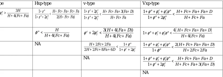
conditions of all pairs of modes of supply are summarized in Table 1. The derivation process is in the appendix A.

Table 1: Ten boundary conditions

n-type m-type Hxp-type v-type Vxp-type

n-type NA 3 2 4( ) a a I H H Fc Fa f + f > + + ₁ 1 _{2 2( )} a a a I H Fc Fa Fc Fa H Fc Fa f f f + _< + + + + + + + + 1 2 3( ) 1 2 c c I a a I H Fc Fa Fa D H Fc Fa f f f f + + _< + + + + + + + + 1 1 2 a c c a I I a a I H Fc Fa Fa D H Fc Fa f f f f f f + + + _< + + + + + + + + m-type NA ) ( 4 Fc Fa H H a + + < j 2 3( 4( )) 4( ) c c I H Fa D H Fc Fa f + f < + + + +

(

)

4 1 4( ) a c c a I I H Fc Fa Fa D H Fc Fa f f f f + + + + + + + < + + Hxp-type NA 2 2 1 2 2 8 6 1 2 a c c I H Fc Fa H Fc Fa D f f f + + _< + + + + + + 1 2( ) 1 2 2 a c c a I I a H Fc Fa Fa D H Fc Fa f f f f j + + + _< + + + + + + + v-type NA ₁ 1 2 3( ) a c c a I I c c I H Fc Fa Fa D H Fc Fa Fa D f f f f f f + + + _< + + + + + + + + + + Vxp-type NA

f. Numerical solutions

We incorporate the difference in iceberg trade costs between components and assembly. While 1+t units need to be shipped to deliver 1 unit of assembled products, 1+αt units need to be shipped out to deliver 1 unit of components. We assume here 0<α<1, i.e., the iceberg trade cost of components is cheaper than that of assembled products. We adopt this assumption for two reasons. First, this assumption sounds reasonable because freights for components are considered to be generally cheaper than that of assembled goods, e.g., engines or chassis versus final cars. Moreover, it is widely known that tariffs are generally lower for intermediate goods than final goods (Olsen’s asymmetry). Secondly, in this symmetric model, firms’ choices come from the trade-off between ‘decomposition (or unbundling)’ costs incorporated as an additional fixed cost versus lower trade cost of components. Thus, unless 0<α<1, ‘decomposition’ never pays off. So, fc > , fa c a

I I

f >f .

We draw a picture of modes of supply in the space of freeness of trade to obtain a testable hypothesis about the relationship between the freeness of trade and the modes of supply. The empirical study in the next section tests the hypothesis.

The area of n-type is the one which simultaneously solves the inequality conditions of the four conditions in the first row of Table 1, which correspond to the equations (A6), (A8), (A12) and (A13). Similarly, we can find the area of each mode of supply by simultaneous inequality conditions derived above. There are four types of freeness of trade in our model, f f f f . To yield figures in two a, c, Ia, Ic

dimensions, we assume fa =rf fc, Ia =rfIc; 0< <r 1. Figure 2 is a numerical solution for one set of parameters. This is the case where all the five modes of supply are within the choice set. Obviously, depending on the parameter values, the picture changes. For example, when ρ takes a high number, such as 0.8, neither v-type nor Vxp-type is within the choice set because the merit of transporting components instead of assembly is small. In Figure 2, when either intra-regional freeness of trade fa or inter-regional freeness of trade a

I

feature does not change depending on the parameter values although the size of area for each mode of supply does change.

g. Intuition

Intuition is straightforward. At a low fa (intra-regional freeness of trade) and a low a I

f (inter-regional freeness of trade) such as A in Figure 2, both of intra-regional trade costs and inter-regional trade costs are high. Thus, it is optimal for firms to avoid transportation both between regions and within regions and set up component and assembly plants in each country, i.e., horizontal FDI (m-type). As the point moves from A to B, f becomes larger while _Ia fa stays low, thus it becomes optimal to take advantage of low inter-regional trade costs and export to the other countries from the home country, i.e., n(national)-type. As the point moves from B to C, fa becomes higher. Because a high fa is associated with a high fc by the parameter ρ (fa =rfc; 0< < ) as abover 1 7, with a sufficiently low value of ρ and D (the decomposition cost) (in the case of Figure 2, ρ=0.5 and D=0.2), it pays for firms to decompose the production process and transport components across regions. Thus, the optimal choice is vertical export platform FDI (Vxp-type). On the way from B to C at intermediate fa, there is an area for vertical FDI (v-type), in which it pays to decompose the production process because of a sufficiently low D, but does not pay to transport the assembled goods (final goods) within regions because fa is not sufficiently high. When the point moves from A to D,

a

f becomes larger while f stays low, thus it becomes optimal to make use of low intra-regional _Ia trade costs and to choose horizontal export platform FDI (Hxp-type). Finally, the movement from D to C (from Hxp-type to Vxp-type) comes from a high a

I

f combined with a sufficiently low value of ρ and D as explained above.

7

Figure 2: Modes of supply in the space of inter-regional freeness of trade (f ) and _Ia intra-regional freeness of trade (fa)

Parameter values: H=1, Fa=0.1, Fc=0.2, D=0.2, ρ=0.5

3. D

ATA

,

EMPIRICAL MODEL AND RESULTS

We use US FDI data from the US Bureau of Economic Analysis (BEA). We have chosen US data because the US is the largest FDI home country and also the US BEA makes the detailed and long-period data publicly available.

a. Descriptive Analysis

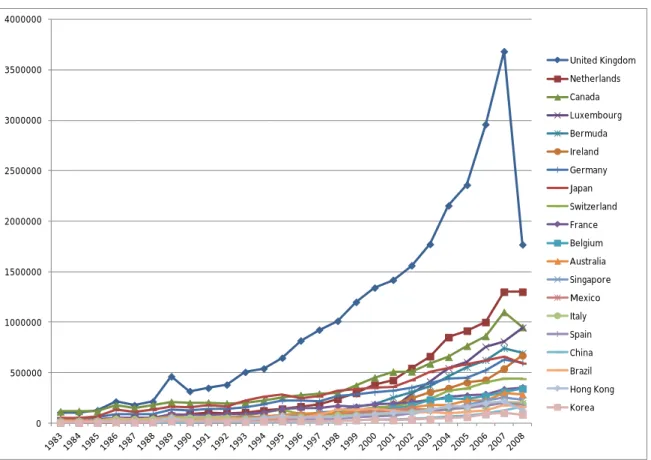
Figure 3 shows the evolution of US FDI stock for the top 20 host countries in terms of its FDI stock in 2008. The United Kingdom is the largest US FDI recipient, having much higher stock amount than the second largest recipient, the Netherlands. To examine the evolution of the other 19 countries more closely, Figure 4 shows the same data excluding the United Kingdom. Countries with strong

A B

D C

increases in FDI stock. Drastic increases in US FDI stock in the Netherlands, Luxembourg and Ireland stand out. The evolution of third country export ratios are in Figure 5. The ratio for the largest US FDI recipient, the United Kingdom, is in the range of 20 to 25%. Luxembourg and Switzerland have the highest ratios ranging from 60% to 80%. Ireland has also a high ratio at the range between 60% and 70%. The ratios of the Netherlands and Belgium are relatively stable at around 55%. The lowest ratios are for Canada and Japan at less than 10%. We notice here that countries that have received the highest amount of US FDI, except the UK, show high ratios. This can be said especially for EU countries.

Figure 3: The evolution of US FDI stock of the top 20 recipient countries, 1983-2008

0 500000 1000000 1500000 2000000 2500000 3000000 3500000 4000000 United Kingdom Netherlands Canada Luxembourg Bermuda Ireland Germany Japan Switzerland France Belgium Australia Singapore Mexico Italy Spain China Brazil Hong Kong Korea

Figure 4: The evolution of US FDI stock of the top 20 recipient countries except UK, 1983-2008 0 200000 400000 600000 800000 1000000 1200000 1400000 19 83 19 84 19 85 19 86 19 87 19 88 19 89 19 90 19 91 19 92 19 93 19 94 19 95 19 96 19 97 19 98 19 99 20 00 20 01 20 02 20 03 20 04 20 05 20 06 20 07 20 08 Netherlands Canada Luxembourg Bermuda Ireland Germany Japan Switzerland France Belgium Australia Singapore Mexico Italy Spain China Brazil Hong Kong Korea

Unit: Million dollars, Source: Author’s computation from US BEA data

Figure 5: The evolution of the third country export ratio of the top 20 US FDI recipient countries, 1983-2008 0.0% 10.0% 20.0% 30.0% 40.0% 50.0% 60.0% 70.0% 80.0% 90.0% 19 83 19 84 19 85 19 86 19 87 19 88 19 89 19 90 19 91 19 92 19 93 19 94 19 95 19 96 19 97 19 98 19 99 20 00 20 01 20 02 20 03 20 04 20 05 20 06 20 07 20 08 United Kingdom Netherlands Canada Luxembourg Bermuda Ireland Germany Japan Switzerland France Belgium Australia Singapore Mexico Italy Spain China Brazil Hong Kong Korea

b. Econometric Analysis

We estimate the following equation.

, 0 1 , 2 , 3 4 5 ,

c t c t c t c t

FDIforThirdCountryExports =b +b MarketPotential +b TradeCost +b% RTA+b%Y+b% H+e

where FDIforThirdCountyExports_{c t,} is the US FDI stock multiplied by the third country export ratio

of host country c at time t. MarketPotential_{c t,} is the market potential values of Mayer (2008)8 of

host country c at time t. We use this variable as a major explanatory variable instead of other variables such as GDP of host countries, since, when choosing locations of their plants, firms look not only at the domestic market of host countries but also at the potential demand coming from the host countries’ neighbours.9 TradeCost_{c t,} is the ratio of trade related cost over goods’ value for host country c at

time t.10 Details for its computation is in Appendix B. This variable corresponds to f , inter-regional _Ia freeness of trade, in the above theoretical model, because it is the trade cost between the US and the host country. RTA is a vector of Regional Trade Agreement dummy. Those dummies are EU dummy, MERCOSUR dummy, ASEAN dummy and NAFTA dummy. This variable corresponds to

a

f , intra-regional freeness of trade, because RTA enhances the freeness of trade. Yis a vector of year dummies. His a vector of host country dummies. e is an iid error. The variables of our interest _{t ,d} are TradeCost_{c t,} and RTA , while the others are control variables. In the above theoretical model,

market sizes are assumed to be constant. However, the actual data must be reflecting the influence of market sizes. Thus, by including the variable, MarketPotential_{c t,} , we are controlling market sizes.

All the variables except dummy variables are in natural log. The data covers the years from 1983 to 2003. The starting year of 1983 comes from the constraint of US FDI data while the end year of 2003

8 I thank Thierry Mayer for kindly sharing with me the market potential data he constructed. 9 Being inspired by the idea of “market potential” by Harris (1954), Head and Mayer (2004) and Mayer (2008) have estimated “market potential” using equations they derived from the New Economic Geography.

10 We compute trade costs as above so that it captures the real trade cost, including transportation, tariff, and insurance, instead of using distance, which does not have variation over time.

comes from the availability of the Market Potential data. Fifty eight countries available from the US FDI data are included. The list of countries is in Appendix C.

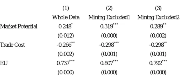
c. Results

Table 2 shows the estimation results. The first column gives the results using the whole data. There is an issue worth being considered. The location choice of natural resource seeking FDI hinges on the availability of natural resources, not on the possibility of third country exports. While we do not have the third country export data by industry as mentioned above, we do have FDI stock data by industry, at least for recent years. Thus, we have run the second regression excluding US FDI recipient countries whose share of mining sector in the total US FDI stock exceeds 50% in the year 2003, the last year of the data for the regression. The mining sector includes Oil and Gas Extraction, Coal Mining, Metal Mining, etc.11 The third column gives results when we exclude more countries by setting the cut-off point at 25%.

As specification tests, we have run pooled regression and panel regression and performed Likelihood ratio test. The likelihood ratio test has rejected the null hypothesis of no systematic difference between pooled regression and panel regressions, leading us to go with the panel. Among the panel regressions, we have performed Hausman tests and chosen between fixed effects or random effects according to the test results.12

In all three cases, the coefficient estimates for the market potential variable is positive and statistically significant, indicating one percent increase of market potential is associated with an increase of 0.248 to 0.319 percent of “FDI stock for third country exports”. The trade cost variable captures inter-regional freeness of trade between the US and the recipient countries. Its coefficient estimates are negative and statistically significant in all three cases, indicating that a one percent increase in trade cost is associated with 0.266 to 0.298 percent decrease of “FDI stock for third country exports”.

11 Industry classification with which the data are available is NAICS 2002.

This is equivalent to saying: one percent increase in inter-regional freeness of trade is associated with 0.266 to 0.298 percent increase in “FDI stock for third country exports”. This result sits well with the theoretical prediction shown above. Namely, as f gets larger (given a sufficiently high level of _Ia fa), firms choose (Vertical) export platform FDI13. The other variable of our interest, Regional Trade Agreement dummies, i.e., EU, MERCOSUR, ASEAN, NAFTA dummies show different coefficient estimates. The EU dummy exhibits large positive coefficient estimates with high statistical significance in all three cases. The MERCOSUR dummy also shows positive coefficient estimates with statistical significance in all three cases. And the numbers are not negligible. The ASEAN dummy’s drastic change from the first column to the second and the third columns comes from the exclusion of Indonesia. Indonesia ranks 24 out of 57 countries and has a high third country export ratio. The mean of third country export ratio of Indonesia is 45.3%. Thus, the first column’s large positive statistically significant coefficient can be interpreted as an Indonesia effect. Once we exclude Indonesia, whose share of mining sector is 65.6%, the coefficient estimates become statistically insignificant. As to the NAFTA dummy, given no large third country neighbours of Canada and Mexico, a statistically insignificant coefficient estimate of NAFTA dummy is not surprising.

Table 2: Estimation results

(1) (2) (3)

Whole Data Mining Excluded1 Mining Excluded2

Market Potential 0.248* 0.319*** 0.289** (0.012) (0.000) (0.002) Trade Cost -0.266** -0.298*** -0.298** (0.002) (0.001) (0.001) EU 0.737*** 0.807*** 0.792*** (0.000) (0.000) (0.000)

13 Here, we put the word “vertical” into the parenthesis because the third country export data do not distinguish between vertical and horizontal FDI. This is unfortunate because a contribution of this paper on theoretical side is the model construction which includes both of horizontal and vertical FDI.

MERCOSUR 0.374* 0.387* 0.382* (0.045) (0.041) (0.042) ASEAN 3.077*** 0.658 0.562 (0.000) (0.369) (0.449) NAFTA -0.309 -0.378 -0.357 (0.128) (0.061) (0.076) Constant 2.575 1.313 1.761 (0.052) (0.252) (0.137) N 946 881 838 p-values in parentheses * _{p < 0.05,} ** _{p < 0.01,} *** _{p < 0.001}

(2) Mining excluded 1: Excluded countries are Nigeria, Egypt, Indonesia, Norway

(3) Mining excluded 2: Excluded countries are Nigeria, Egypt, Indonesia, Norway, Peru, Russia, Ecuador, United Arab Emirates

4. C

ONCLUSION

This paper contributes a model that accounts for “export platform” FDI – a form of FDI that is common in the data but rarely discussed in the theoretical literature. Unlike the previous literature, this paper’s theory nests all the typical modes of supply, including exports, horizontal and vertical FDI, horizontal and vertical export platform FDI. The theory yields the testable hypothesis that a decrease in inter-regional or intra-regional trade costs induces firms to choose the export platform FDI. The empirical part of the paper provides descriptive statistics, which point to large proportions of third country exports of US FDI, and an econometric analysis, whose results are in line with the model’s predictions. A strong positive impact of the EU dummy on the export platform FDI suggests policy implications for nations seeking to attract FDI More precisely, the easier access to third countries’ markets brought about by regional trade agreements shows to be a strong determinant of the locational decisions of US firms. This shows a non-obvious rarely mentioned benefit of smaller countries joining RTAs.

This paper abstracts away from the issue of cost difference for the sake of constructing a parsimonious model, and as a result, focus on the proximity-concentration trade-off with unbundling

costs. This model may well explain the export platform FDI in EU countries, but is not suitable to account for the export platform FDI inflows to developing countries, such as Japanese FDI into Mexico, where the motive of production cost saving must be involved. To incorporate production cost motive or construct another model for that purpose is a future work to be done.

R

EFERENCES

Ando, M., Kimura, F.,(2005a). The Formation of International Production and Distribution Networks in East Asia. In : Ito, T., Rose, A. (Eds.), International Trade in East Asia, NBER-East Asia Seminar on Economics, vol. 14., National Bureau of Economic Research

Ando, M., Kimura, F., (2005b). The Economic Analysis of International Production/Distribution Networks in East Asia and Latin America: The Implication of Regional Trade Agreements., Business and Politics, vol. 7., issue 1

Baldwin, R., Forslid, R., Martin, P., Ottaviano, G., Robert-Nicoud, F., 2003. Economic Geography and Public Policy. Princeton University Press

Baltagi, B., Egger, P., Pfaffermayr, M. 2007. Estimating models of complex FDI: Are there third-country effects?, Journal of Econometrics, 140 260-281

Bergstrand, J., Egger, P. 2007. A knowledge-and-physical-capital model of international trade flows, foreign direct investment, and multinational enterprises, Journal of International Economics, vol. 73(2) 278-308, November

Blonigen, B., Davies, R., Waddell, G., Naughton, H. 2007. FDI in space: Spatial autoregressive relationships in foreign direct investment, European Economic Review, 51 1303-1325

Ekholm, K., Forslid, R., Markusen, J., 2007. Export Platform Foreign Direct Investment., Journal of the European Economic Association, 5(4), 776-795

Feinberg, S., Keane, M., 2006. Accounting for the Growth of MNC-Based Trade Using a Structural Model of U.S. MNCs., American Economic Review, vol.96, No.5, pp.1515-1558

Greenaway, D. and Kneller, R., 2007. Firm heterogeneity, exporting and foreign direct investment., The Economic Journal 117 (February) F134-F161

Grossman, G., Helpman, E., Szeidl, A., 2006. Optimal integration strategies for the multinational firm., Journal of International Economics, 70, 216-238

Hanson, G.H., Mataloni, R.J., Slaughter, M.J., 2001. Expansion strategies of U.S. multinational corporations. Brookings Trade Forum 2001, pp. 245– 294.

Harris, C. 'The Market as a Factor in the Localization of Industry in the United States', Annals of the Association of American Geographers, Vol. 44, No. 4 (Dec., 1954), pp.315-348

Head, K., Mayer, T., 2004 Market Potential and the Location of Japanese Investment in the European Union., The Review of Economics and Statistics, 86(4), 959-972

Helpman, E. and Krugman, P., 1985. Market Structure and Foreign Trade. MIT Press

Navaretti, G.B. and Venables, A. (2004)Multinational Firms in the World Economy. (New Jersey, USA: Princeton University Press)

Markusen, J., 2002. Multinational Firms and the Theory of International Trade. MIT press Mayer, T., 2008. Market Potential and Development., CEPR Discussion Paper No. 6798 Motta, M. and Norman, G. (1996). Does economic integration cause foreign direct investment?,

International Economic Review, vol. 37 (4), pp. 757–83.

Murázová, M., Neary, P., 2010. Firm Selection into Export-Platform Foreign Direct Investment. CEPR Discussion Paper.

Neary, P., 2009. Trade Costs and Foreign Direct Investment., International Review of Economics & Finance. Vol. 18(2), pages 207-218, March

Yeaple, S., 2003. The complex integration strategies of multinationals and cross country

dependencies in the structure of foreign direct investment, Journal of International Economics, 60 293-314

Appendix A:

Operating profit

Firm k in county i maximizes

(

)

k k k k

i pi ci qi

p = - (A1)

where p, c, q represent price, marginal cost, and quantity respectively. The first order condition yields the Lerner condition.

(

1 1

)

k k k i i i p - e =c (A2) where k i

e is the firm’s perceived elasticity of demand. Plugging (A2) into (A1) gives

k k k k i p qi i i

p = e (A3)

Denoting the firm’s market share as k k k i i i i

s º p q R where R is market size of country i, (A3) _i

becomes

k k k

i s Ri i i

p = e (A4)

Assuming that each firm’s perceived elasticity of demand depends only on the market share of the firm, e_ik = ë ûeé ùs_ik , (A4) becomes

k k k

i s Ri i si

p = eé ù_{ë û} (A5)

Derivation of the “erosion” effect

Without τ, we have /

pq

p = e

Because of the Dixit-Stiglitz CES utility function, with τ, the equilibrium sales quantity is: 1 1 E q p P s s s t - -=

1 1 E p p P s s s p t - - e -= ×

With the assumption of identical firms, this becomes:

1 1 1 E p P s s s p t - - s -= Since 1 1 1 1 1 1 1 p p p P p np n s s s s s s - -

-- =

å

- = - = due to identical firms, and also because

px s

E

º

Since E=npx due to identical firms, 1 px s npx n = = Thus, 1 sE s p t₌ - s Since f tº 1-s, p f= sE s q.e.d.

Assuming the cost function, c=wz

where w is wage and z is intermediate inputs.

If we transport final goods, the marginal cost becomes c=t_a

( )

wz . And the above derivation applies. If we transport intermediate goods, the cost becomes c=t_a

(

w

( )

t_cz

)

.

Due to the multiplicative term, the operating profit becomes p f f= _{a c}sE s

Derivation of the boundary conditions

Between n-type and m-type

The equilibrium condition of firms choosing n-type instead of m-type is that n-type yields zero profits while m-type yields negative profits. Thus, the boundary condition can be found as14:

) ( / / / / S R S R S R H Fc Fa SR a _Ia _Ia n = + + + - + + P s j s j s j s =0

14 The only endogenous variable in the equations is market share S. So, we solve the equality condition for S and then by plugging this S into the

0 ) ( / ) 2 1 ( + + - + + = ÛSR ja j_Ia s H Fc Fa Solving for S, ) 2 1 ( ) ( a I a R Fa Fc H S j j s + + + + = Û

Plugging this into the inequality condition of P , m

0 )) ( 4 ( ) 2 1 ( ) ( 4 - + + < + + + + = P R H Fc Fa R Fa Fc H a I a m s j j s 3 2 4( ) a a I H H Fc Fa f f Û + > + + (A6)

Analogously, the boundary conditions of other pairs of modes of supply are: Between m-type and Hxp-type

4( )

a H

H Fc Fa

f <

+ + (A7)

Between n-type and v-type

1 2 3( ) 1 2 c c I a a I H Fc Fa Fa D H Fc Fa f f f f + + _< + + + + + + + + (A8)

Between v-type and Vxp-type

1 1 2 3( ) a c c a I I c c I H Fc Fa Fa D H Fc Fa Fa D f f f f f f + + + + + + + < + + + + + + (A9)

Between m-type and v-type

3( 4( )) 2 4( ) c c I H Fa D H Fc Fa f + f < + + + + (A10)

Between v-type and Hxp-type

1 a 2 2

H Fc Fa

f

Between n-type and Hxp-type 1 1 2 2( ) a a a I H Fc Fa Fc Fa H Fc Fa f f f + _< + + + + + + + + (A12)

Between n-type and Vxp-type

1 1 2 a c c a I I a a I H Fc Fa Fa D H Fc Fa f f f f f f + + + + + + + < + + + + (A13)

Between m-type and Vxp-type

(

)

4 1 4( ) a c c a I I H Fc Fa Fa D H Fc Fa f f f f + + + + + + + < + + (A14)

Between Hxp-type and Vxp-type

1 2( ) 1 2 2 a c c a I I a H Fc Fa Fa D H Fc Fa f f f f f + + + _< + + + + + + + (A15)

Appendix B:

We have used US import data provided by The Center for International Data at UC Davis. The variable “charge” in the data represents trade related costs except import duty. For the years prior to 1989, the data do not include “charge”. Thus, we have computed the “charge” as “cifvalue” minus “cusvalue”, i.e., CIF value – FOB value. Since the data are at 7 or 10 digit product code depending on years, we have computed total “cusvalue”, total “charge” and total “duty” by summing over product codes for each pair of years and partner countries. Finally we defined the trade cost as the total “charge” + total “duty” divided by the total “cusvalue”.

Appendix C:

US FDI econometric analysis, List of countries

Argentina Greece Panama

Australia Guatemala Peru

Austria Honduras Philippines

Bahamas Hong Kong Poland

Barbados Hungary Russia

Belgium India Saudi Arabia

Bermuda Indonesia Singapore

Brazil Ireland South Africa

Canada Israel Spain

Chile Italy Sweden

China Jamaica Switzerland

Colombia Japan Thailand

Costa Rica Korea, Republic of Trinidad and Tobago Czech Republic Malaysia Turkey

Denmark Mexico United Arab Emirates

Ecuador Netherlands United Kingdom

Egypt Netherlands Antilles Venezuela

Finland New Zealand

France Nigeria