Allocation efficiency in China : an extension
of the dynamic Olley-Pakes productivity
decomposition
著者
Hashiguchi Yoshihiro
権利
Copyrights 日本貿易振興機構(ジェトロ)アジア
経済研究所 / Institute of Developing
Economies, Japan External Trade Organization
(IDE-JETRO) http://www.ide.go.jp
journal or
publication title
IDE Discussion Paper
volume
544
year
2015-11-01
INSTITUTE OF DEVELOPING ECONOMIES
IDE Discussion Papers are preliminary materials circulated to stimulate discussions and critical comments
Keywords: Misallocation, Firm-level productivity, Structural estimation, China JEL classification: D24, O47
* OECD Paris ([email protected])
Institute of Developing Economies ([email protected])
IDE DISCUSSION PAPER No. 544
Allocation Efficiency in China: An
Extension of the Dynamic Olley-Pakes
Productivity Decomposition
Yoshihiro HASHIGUCHI*
November 2015
Abstract
This paper develops a quantitative measure of allocation efficiency, which is an extension of the dynamic Olley-Pakes productivity decomposition proposed by Melitz and Polanec (2015). The extended measure enables the simultaneous capture of the degree of misallocation within a group and between groups and parallel to capturing the contribution of entering and exiting firms to aggregate productivity growth. This measure empirically assesses the degree of misallocation in China using manufacturing firm-level data from 2004 to 2007. Misallocation among industrial sectors has been found to increase over time, and allocation efficiency within an industry has been found to worsen in industries that use more capital and have firms with relatively higher state-owned market shares. Allocation efficiency among three ownership sectors (state-owned, domestic private, and foreign sectors) tends to improve in industries wherein the market share moves from a less-productive state-owned sector to a more productive private sector.
The Institute of Developing Economies (IDE) is a semigovernmental, nonpartisan, nonprofit research institute, founded in 1958. The Institute merged with the Japan External Trade Organization (JETRO) on July 1, 1998.
The Institute conducts basic and comprehensive studies on economic and related affairs in all developing countries and regions, including Asia, the Middle East, Africa, Latin America, Oceania, and Eastern Europe.
The views expressed in this publication are those of the author(s). Publication does not imply endorsement by the Institute of Developing Economies of any of the views expressed within.
INSTITUTE OF DEVELOPING ECONOMIES (IDE), JETRO 3-2-2, WAKABA,MIHAMA-KU,CHIBA-SHI
CHIBA 261-8545, JAPAN
©2015 by Institute of Developing Economies, JETRO
Allocation E
fficiency in China: An Extension of the
Dynamic Olley-Pakes Productivity Decomposition
∗
Yoshihiro HASHIGUCHI
†OECD Paris
Institute of Developing Economies
November 2015
Abstract
This paper develops a quantitative measure of allocation efficiency, which is an
ex-tension of the dynamic Olley-Pakes productivity decomposition proposed by Melitz and Polanec (2015). The extended measure enables the simultaneous capture of the degree of misallocation within a group and between groups and parallel to capturing the contribution of entering and exiting firms to aggregate productivity growth. This measure empirically assesses the degree of misallocation in China using manufacturing firm-level data from 2004 to 2007. Misallocation among industrial sectors has been found to increase over time,
and allocation efficiency within an industry has been found to worsen in industries that use
more capital and have firms with relatively higher state-owned market shares. Allocation
efficiency among three ownership sectors (state-owned, domestic private, and foreign
sec-tors) tends to improve in industries wherein the market share moves from a less-productive state-owned sector to a more productive private sector.
Keywords: Misallocation, Firm-level productivity, Structural estimation, China
JEL classification: D24, O47
∗I would like to thank participants at the Fudan University Workshop 2014, the OECD Mini-Conference 2014,
and the Institute of Developing Economies Workshop 2014 for their constructive comments. All remaining errors are my own.
†Address: 2, Rue Andr´e-Pascal 75775 Paris CEDEX 16, France.
1
Introduction
Recent studies argued that the allocation of production resources among firms or sectors is a key driver behind the growth of aggregate total factor productivity (TFP) (Restuccia and Roger-son, 2008; Hsieh and Klenow, 2009; Bartelsman et al., 2013; Collard-Wexler and De Loecker, 2015). Their argument is that the shift in production resources from less productive to more productive units yields an increase in aggregate TFP and that resource allocation efficiency is crucial to explaining countries’ aggregate TFP. A well-functioning market economy can allo-cate more production resources to more productive businesses. Because developing economies are generally found to have lower allocation efficiency than developed economies, improving resource allocation is expected to increase their aggregate TFP and GDP per capita. Therefore, developing an appropriate measure of allocation efficiency and theoretically and empirically investigating the sources of misallocation are crucial to implementing better economic policies. In this paper, the author develops an extended quantitative measure of allocation efficiency. Two types of empirical measures of allocation efficiency have been used in previous studies: (1) the dispersion of firm-level productivity (Hsieh and Klenow, 2009) and (2) the covariance between a firm’s market share and productivity (Olley and Pakes, 1996; Collard-Wexler and De Loecker, 2013; Melitz and Polanec, 2015). According to Bartelsman et al. (2013), the covariance measure is a robust theoretical and empirical measure to assess the effect of misallo-cation. The covariance measure was originally proposed by Olley and Pakes (1996), Melitz and Polanec (2015) extended it to capture the contributions of entering and exiting firms, calling it the dynamic Olley-Pakes (OP) productivity decomposition. However, the dynamic and non-dynamic (i.e., original) OP decomposition do not capture allocation efficiency between groups (e.g., industrial sectors, ownership groups); they only capture allocation efficiency within a group. This paper attempts to extend the OP decomposition to a multi-group version to simul-taneously capture the degree of allocation efficiency within a group and between groups and parallel to capturing the contribution of entering and exiting firms.
The extended productivity decomposition method is applied to China’s manufacturing firm-level data from 2004 to 2007. Several scholars estimated the degree of allocation efficiency in China. However, some debate has occurred over its recent trend. For example, Hsieh and Klenow (2009) used manufacturing firm-level data from 1998 to 2005 to measure the degree of misallocation. They found that misallocation within an industry tended to decline over time. Meanwhile, Chen et al. (2011) used industry-level data from 1980 to 2008 and found that factor reallocation played a substantial role in increasing aggregate productivity from 1980 to 2000; however, after 2001, they found that allocation efficiency worsened and contributed to decreasing productivity growth. Brandt et al. (2013) also used industry-level data by province from 1985 to 2007 and found that misallocation within provinces declined between 1985 and 1997 but increased in the last 10 years. Has China’s allocation efficiency worsened since the 2000s? What is the extent of its allocation efficiency among industrial sectors and ownership groups? The investigations into China’s allocation efficiency remain insufficient.
This paper addresses these questions using the extended measure of allocation efficiency. The empirical analysis has two steps. First, firm-level productivity is estimated using a struc-tural estimation method proposed by Gandhi et al. (2013). Second, the productivity decompo-sition method is exploited to quantify the effect of misallocation on aggregate manufacturing productivity. Hence, misallocation between industrial sectors is revealed as increasing over time, and changes in misallocation between industrial groups have a more significant effect
on aggregate TFP growth than effect of misallocation changes within an industry. Misalloca-tion within an industry is found to increase in industries that use more capital and have firms with relatively higher state-owned market shares. However, allocation efficiency between three ownership sectors (state-owned, domestic private, and foreign sectors) tends to improve in in-dustries in which the market share moves from a less-productive state-owned sector to a more productive private sector. However, this efficiency tends to worsen in industries in which 1) the state-owned sector’s TFP increases on relative basis despite decreases in its market share or 2) the private sector’s TFP does not grow compared with other sectors despite increases in its market share.
The remainder of this paper is structured as follows. Section 2 describes the measure of allocation efficiency used in this study. Section 3 describes the TFP estimation procedure, and Section 4 presents the data sources and estimation results of productivity. Section 5 reports the allocation efficiency in China, and Section 6 concludes.
2
Measure of Allocation E
fficiency
The measure of allocation efficiency used in this paper is based on a productivity decomposi-tion method originally developed by Olley and Pakes (OP; 1996) and extended by Melitz and Polanec (MP; 2015) to a dynamic version. Sections 2.1 and 2.2 review the OP and MP meth-ods, and Section 2.3 describes the extended version of their methods. Section 5.2 reports the empirical results of China’s allocation efficiency.
2.1
Olley-Pakes Decomposition
Let us consider aggregate productivity (Φt), which is defined as the weighted average of
firm-level productivity: Φt =
∑
i∈Ωt sitϕit, whereΩtis the set of firms at time t,ϕitis the firm-level log
TFP, and sitis firm i’s share of output at time t. Olley and Pakes (1996) showed that aggregate
productivity can be decomposed into the following two parts:
Φt = ∑ i∈Ωt sitϕit = 1 Nt ∑ i∈Ωt ϕit+ ∑ i∈Ωt sit− 1 Nt ∑ ι∈Ωt sιt ϕit− 1 Nt ∑ ι∈Ωt ϕιt = µt+ covt (1)
where µt represents the unweighted mean productivity and covt is proportional to the
covari-ance between market shares and productivity. covt represents the magnitude of allocation e
ffi-ciency because it increases as more-productive firms have higher market shares, and conversely, it decreases as less productive firms have higher market shares. Olley and Pakes (1996) used plant-level panel data on the U.S. telecommunications equipment industry from 1974 to 1987 to estimate plant-level productivity for the industry and then exploited it to calculate OP decom-position. They found that the unweighted mean productivity (µt) did not change much since
1975, but the covariance term increased from 0.01 in 1974 to 0.32 in 1987. They concluded that a factor reallocation occurred from less-productive to more-productive plants.
2.2
Dynamic Olley-Pakes Decomposition
Melitz and Polanec (2015) extended the OP decomposition to capture the contribution of en-tering and exiting firms in aggregate productivity, which is called the dynamic Olley-Pakes productivity decomposition. They showed that the difference in the aggregate log TFP at times 1 and 2 (∆Φ = Φ2 − Φ1) can be decomposed into the following parts: (1) unweighted TFP
of firms surviving during the period, (2) the OP’s covariance term calculated using surviving firms’ log TFP and market shares, and (3) the contribution of entering and exiting firms during the period.
The dynamic Olley-Pakes (DOP) decomposition is derived as follows. First, the aggregate log TFP at time 1 (Φ1) is decomposed into surviving firms’ log TFP at time 1 and exiting firms’
log TFP at time 1: Φ1 = ∑ i∈ΩS si1ϕi1+ ∑ i∈ΩX si1ϕi1 = ΦS 1 + s X 1 ( ΦX 1 − Φ S 1 ) , (2)
whereΩS andΩX denote the sets of surviving and exiting firms during the period andΦS
1 and
ΦX
1 are the aggregate log TFPs at time 1 for surviving and exiting firms, respectively:
ΦS 1 = ∑ i∈ΩS si1 ∑ ι∈ΩS sι1ϕ i1, ΦX1 = ∑ i∈ΩX si1 ∑ ι∈ΩX sι1ϕ i1, sX1 = ∑ i∈ΩX si1.
Similarly, the aggregate log TFP at time 2 is decomposed into surviving firms’ log TFP at time 2 and entering firms’ log TFP at time 2:
Φ2 = ∑ i∈ΩS si2ϕi2+ ∑ i∈ΩE si2ϕi2 = ΦS 2 + s E 2 ( ΦE 2 − Φ S 2 ) , (3)
whereΩE denotes the set of entering firms during the period andΦS2 andΦE2 are the aggregate log TFPs at time 2 for surviving firms and entering firms, respectively:
ΦS 2 = ∑ i∈ΩS si2 ∑ ι∈ΩS sι2ϕ i2, ΦE2 = ∑ i∈ΩE si2 ∑ ι∈ΩE sι2ϕ i2, sE2 = ∑ i∈ΩE si2.
Applying the OP decomposition toΦS
t (t= 1, 2) yields: ΦS t = 1 NS ∑ i∈ΩS ϕit+ ∑ i∈ΩS ∑ sit ι∈ΩS sιt − 1 NS ∑ i∈ΩS sit ∑ ι∈ΩS sιt ϕit− 1 NS ∑ i∈ΩS ϕit = µS t + cov S t, (4)
where NS is the number of firms surviving during the period,µSt is the unweighted mean
pro-ductivity of surviving firms, and covSt represents the magnitude of allocation efficiency among surviving firms. Substituting Equation (4) in Equations (2) and (3) and taking the difference of the aggregate log TFP (∆Φ = Φ2− Φ1) results in the DOP decomposition as follows:
∆Φ = ∆µS + ∆covS + sE 2(Φ E 2 − Φ S 2)+ s X 1(Φ S 1 − Φ X 1)
where ∆µS = µS 2 − µ S 1, ∆cov S = covS 2 − cov S 1, ent = s E 2(Φ E 2 − Φ S 2), and ext = s X 1(Φ S 1 − Φ X 1).
The first term on right-hand side is the change in the unweighted average log TFP for surviving firms. The second term is the change in the covariance, which indicates the change in the magnitude of allocation efficiency among surviving firms. The contributions of entering and exiting firms appear in ent and ext, respectively, both of which are evaluated in comparison with the productivity of surviving firms as follows:
ent ⋚ 0 when ΦE2 ⋚ ΦS2, ext ⋚ 0 when ΦS1 ⋚ ΦX1.
Thus, the DOP decomposition method allows us to identify the contributions of entering and exiting firms.
Melitz and Polanec (2015) used firm-level panel data from the Slovenian manufacturing sector from 1995 to 2000 to estimate the parameters of a production function for the industry and then calculated the DOP decomposition using the estimated log TFP and the log of labor productivity. They found that the aggregate log TFP change (∆Φ) from 1995 to 2000 is 0.4013 and is decomposed into the unweighted mean productivity for surviving firms (∆µS = 0.2758),
the covariance term change (∆covS = 0.0955), and the contributions of entering and exiting firms (ent = 0.0021, ext = 0.0279). Their results indicate that the improvement in allocation efficiency added 10 percentage points to aggregate TFP growth during the five years.
2.3
Extension of the OP and Dynamic OP Decompositions
The OP and DOP decompositions allow us to quantify the degree of allocation efficiency within a group (e.g., an industrial sector). However, these quantifications can be augmented to a multi-group version to simultaneously capture the degree of allocation efficiency within a group and between groups. This section shows the augmented version of the OP and DOP decomposition.
2.3.1 Augmented OP (AOP) Decomposition
Let us consider that the number of groups is J and aggregate productivity is represented as:
Φt = ∑J j=1wjt ∑ i∈Ωjt sit wjt ϕit =∑Jj=1wjtµ˜jt,
whereΩjtis the set of firms in group j at time t, wjtis group j’s output share at time t, and ˜µjt=
∑
i∈Ωjt(sit/wjt)ϕitis the weighted average log TFP for group j. Applying the OP decomposition
to the above equation yields:
Φt = 1 J ∑J j=1µ˜jt+ ∑J j=1 ( wjt− 1 J ∑J κ=1wκt ) ( ˜ µjt− 1 J ∑J κ=1µ˜κt ) = 1 J ∑J j=1µ˜jt+ ˜covt, (6)
where ˜covt represents the magnitude of inter-group allocation efficiency. This paper defines the
The ˜µjtin the within-effect can be decomposed as: ˜ µjt = 1 Njt ∑ i∈Ωjt ϕit+ ∑ i∈Ωjt sit wjt − 1 Njt ∑ ι∈Ωjt sιt wjt ϕit− 1 Njt ∑ ι∈Ωjt ϕιt = µjt+ covjt, (7)
where Njtis the number of firms in group j at time t. Substituting Equation (7) in Equation (6)
yields the augmented OP (AOP) decomposition as follows:
Φt = 1 J ∑J j=1µjt+ 1 J ∑J j=1covjt | {z } Within effect + |{z}cov˜ t Between effect . (8)
The first term in Equation (8) is the unweighted mean productivity, and covjtand ˜covt represent
the degree of allocation efficiency within group j and between groups, respectively. When
J = 1, Equation (8) reduces to the original OP decomposition. Taking the difference in Equation
(8) yields: ∆Φ = 1 J ∑J j=1∆µj+ 1 J ∑J j=1∆covj+ ∆ ˜cov. (9)
2.3.2 Augmented Dynamic OP (ADOP) Decomposition
The dynamic OP decomposition is also extended to a multi-group case. First, as in the case of the OP decomposition, the aggregate log TFP at time 1 can be decomposed into within- and between-effects: Φ1 = 1 J ∑J j=1µ˜j1+ ˜cov1, (10) where ˜µj1 = ∑ i∈Ωj1(si1/wj1)ϕi1 and ˜cov1 = ∑J
j=1(wj1− w∗1)( ˜µj1 − ˜µ∗1). w∗1 and ˜µ∗1 denote simple
averages of wj1 and ˜µj1, respectively. The weight ai j1 = si1/wj1can be written as
∑ i∈Ωj1 ai j1 = ∑ i∈ΩS j ai j1+ ∑ i∈ΩX j ai j1 = aS j1+ a X j1 = 1. whereΩS j andΩ X
j denote the sets of surviving and exiting firms for group j, respectively. They
can be decomposed into the weighted average log TFP of surviving firms and the contribution of exiting firms: ˜ µj1 = ∑ i∈ΩS j ai j1 aS j1 ϕi1+ aXj1 i∑∈ΩX j ai j1 aX j1 ϕi1− ∑ i∈ΩS j ai j1 aS j1 ϕi1 = ΦS j1+ a X j1 ( ΦX j1− Φ S j1 ) = ΦS j1− extj, (11) whereΦS j1andΦ X
j1denote the weighted average log TFP of surviving and exiting firms for group
j, respectively, and extj = aXj1
( ΦS j1− Φ X j1 )
j’s aggregate productivity ˜µj1. By exploiting the OP decomposition method, the first term of
Equation (11) can be decomposed as:
ΦS j1 = 1 NSj1 ∑ i∈ΩS j ϕi1+ ∑ i∈ΩS j ai j1 aSj1 − 1 NSj1 ∑ ι∈ΩS j aι j1 aSj1 ϕi1− 1 NSj1 ∑ ι∈ΩS j ϕι1 = µS j1+ cov S j1, (12) whereµS
j1 is the simple average log TFP of surviving firms at time 1 and cov S
j1 is the degree of
allocation efficiency within group j at time 1. Substituting Equations (12) and (11) in Equation (10) yields the following decomposition:
Φ1= 1 J ∑J j=1 ( µS j1+ cov S j1− extj ) | {z } Within effect + |{z}cov˜ 1 Between effect . (13)
Similarly, the aggregate log TFP at time 2 can be decomposed as follows:
Φ2 = 1 J ∑J j=1µ˜j2+ ˜cov2 = 1 J ∑J j=1 ( ΦS j2+ a E j2 ( ΦE j2− Φ S j2 )) + ˜cov2 = 1 J ∑J j=1 ( µS j2+ cov S j2+ entj ) | {z } Within effect + |{z}cov˜ 2 Between effect , (14) where entj = aEj2 ( ΦE j2− Φ S j2 )
indicates the contribution of entering firms to aggregate produc-tivity ˜µj2.
Finally, taking the difference between Φ1 and Φ2, the augmented dynamic OP (ADOP)
decomposition is obtained: ∆Φ = 1 J ∑J j=1 ( ∆µS j + ∆cov S j + entj+ extj ) | {z } Within effect + ∆ ˜|{z}cov Between effect (15) where∆covS
j represents the changes in allocation efficiency among surviving firms within group
j and∆ ˜cov represents the changes in allocation efficiency between groups. When J = 1, Equa-tion (14) reduces to the original dynamic OP decomposiEqua-tion. The definiEqua-tion of∆ ˜cov in Equation (15) is the same as that of Equation (9).
In this paper, Equations (9) and (15) are used to decompose China’s aggregate productivity and investigate the magnitude of allocation efficiency. The empirical results are described in Section 5. Before reporting the results, the next section explains how to measure firm-level productivity (ϕit).
3
Production Function Estimation
Having clarified the measure of allocation efficiency in the previous section, showing the mea-sure of firm-level productivity is required. This paper employs the structural estimation method
proposed by Gandhi et al. (GNR; 2013) to measure China’s firm-level productivity. This method is built on the recent literature on production function estimation, such as Olley and Pakes (1996), Levinsohn and Petrin (LP; 2003), and Ackerberg et al. (ACF; 2006). Following GNR (2013), this section describes the framework of firm behavior and shows the identification strategy of the production function.
3.1
Model of Firm Behavior
Let us consider that firm i operates through discrete time t and produces output using labor Lit,
capital Kit, and intermediate inputs Mit. The firm’s anticipated output Qitis assumed to depend
on these inputs, and the anticipated productivity level ωit. ωit represents a firm’s technology,
information, knowledge, or situation that affects its productivity; this can be observed by firm
i, but not by the econometrician. For example,ωitrepresents business management differences,
deviations from expected machine breakdown rates in a particular period, or labor management problems.
At the beginning of each period, firm i can observeωit, which affects current and future
input decisions. The relationship between Qitand the inputs in period t is expressed as:
Qit= F(Kit, Lit, Mit) exp{ωit}, (16)
Yit = Qitexp{εit}, (17)
∴ Yit = F(Kit, Lit, Mit) exp{ωit+ εit}, (18)
where F(·) is a production function and Yitis the measured output observed by the
econometri-cian. The difference between Qitand Yitisεit, representing an unanticipated productivity shock
and/or measurement error that cannot be observed by firm i before making period t’s input de-cisions. TFP is defined as exp{ωit+ εit}. Taking the logarithm for both sides of Equation (18)
yields:
yit = f (kit, lit, mit)+ ωit+ εit, (19)
log TFPit = ωit+ εit,
where the lower-case letters denote the logs of their upper-case letters. Identifying f (kit, lit, mit)
is required to estimate TFP.
As in OP (1996), LP (2003), ACF (2006), and GNR (2013), assumptions about the dynamics of productivity and the timing of input decisions are required to identify the production function. First, the anticipated productivity ωit evolves over time according to the first-order Markov
process and is decomposed into its conditional expectation given all information (Θi,t−1) known
by the firm at t− 1 and a residual (ξit). Thus,ωitcan be expressed as:
ωit = E(ωit | Θi,t−1)+ ξit
= E(ωit | ωi,t−1)+ ξit
= g(ωi,t−1)+ ξit,
(20)
whereξitis, by definition, uncorrelated to g(ωi,t−1) because it is defined as new information not
available in period t− 1, which is frequently referred to as an innovation at t. The innovation ξit
and the ex post shock εit are assumed to be mean zero random variables. Equation (19) can be
rewritten as:
For the timing of input decisions, as with GNR, labor and capital inputs at t are assumed to be decided at or before t−1, implying that these inputs are quasi-fixed inputs and that adjustment costs exist in labor and capital (e.g., hiring/firing, job training, or machine installation costs). Under these timing assumptions, labor and capital inputs can be regarded as state variables for firms, and they are orthogonal to the innovation at t, i.e., E(ξit | kit, lit) = 0. This moment
condition is required to identify the elasticities associated with labor and capital inputs.
The intermediate input Mitis assumed to be a flexible input, which is variable in each period
and does not have dynamic implications. Therefore, its level at t does not affect the firm’s profit in the future. At the beginning of each period, given the levels of labor, capital inputs, andωit,
firm i chooses the level of Mit. Consequently, Mit is an implicit function of Kit, Lit,ωit, and the
output and intermediate input prices. This result implies two points. First, Mitis an endogenous
variable because it partly depends on ωit, which cannot be observed by the econometrician.
Second, no source of cross-sectional variation exists in Mitother than the remaining inputs: Kit,
Lit, and ωit. In other words, Mit is “collinear” with the other productive inputs. As a result,
the identification problem arises with flexible input, which was pointed out by Marschak and Andrews (1944), Bond and S¨oderbom (2005), ACF (2006), and GNR (2013). To address this problem, ACF (2006) suggested strategies using value-added production functions to remove flexible inputs, such as an intermediate input, whereas Wooldridge (2009) proposed the use of lagged inputs decisions as instruments. However, GNR (2013) argued that these solutions are incomplete and showed that TFP estimates based on value-added functions have significant bias and that Wooldridge’s approach does not solve the collinearity problem. GNR (2013) proposed an alternative approach to solving the identification problem based on gross output production functions, including both quasi-fixed inputs and flexible inputs. This paper employs their identification strategy.
3.2
Identification
For estimation purposes, a translo-type production function is used for f (kit, lit, mit):
yit= βkkit+ βllit+ βmmit
+ βkkkit2+ βlll2it+ βmmm2it
+ βklkitlit+ βlmlitmit+ βkmkitmit
+ ωit+ εit,
(22)
where a constant term of the production function is included inωit. GNR’s identification
strat-egy consists of two stages. The first stage involves estimating parameters associated with the intermediate input by using the firm’s first-order condition with respect to Mit under perfect
competition in the input and output markets:
PtFM(Kit, Lit, Mit) exp{ωit} = ρt, (23)
where FM(·) = ∂F(·)/∂Mit, and Pt and ρt denote the output and intermediate input prices,
the intermediate input: Sit= ρtMit PtYit = PtFM(Kit, Lit, Mit) Mit PtYit exp{ωit} = FM(Kit, Lit, Mit) Mit F(Kit, Lit, Mit) exp{ωit+ εit} exp{ωit} = FM(Kit, Lit, Mit) Mit F(Kit, Lit, Mit) 1 exp{εit} = G(Kit, Lit, Mit) 1 exp{εit} , (24)
where G(·) is the elasticity of the anticipated output with respect to Mit. Taking the logarithm
of both sides of Equation (24) enables the share equation to be rewritten as:
sit = log Γit− εit, (25)
where sit = log SitandΓit= G(Kit, Lit, Mit). Becauseεitis the ex post shock that is, by definition,
uncorrelated with the input decisions, logΓitcan be identified by the non-parametric regression
of sit on logΓit.1) The estimates ˆΓit and ˆεit = sit− log ˆΓitare used to identify the parameters in
Equation (22). Based on the production function in Equation (22), the elasticity associated with
Mitcan be written as:
eit(θ1)= βm+ βmm2mit+ βkmkit+ βlmlit, (26)
whereθ1 = (βm, βmm, βkm, βlm)′. Given the observation, because Equation (26) depends only on
the parameters associated with Mit, we can recoverθ1 by minimizing the distance between ˆΓit
and eit(θ1): min θ1 ∑ t ∑ i [ ˆ Γit− eit(θ1) ]2 . (27)
The second stage identifies the remaining parameters associated with kitand litby using the
moment conditions E(ξit | kit, lit) = 0. Given the estimates for ˆθ1 and ˆεit obtained in the first
stage,ωitcan be written as:
ωit= yit− ˆβmmit− ˆβmmm2it− ˆβkmkitmit− ˆβlmlitmit− ˆεit
− βkkit− βllit− βkkkit2− βlll2it− βklkitlit
= yit− z1itθˆ1− z2itθ2− ˆεit
= ˜yit− z2itθ2
(28)
where ˜yit= yit− z1itθˆ1− ˆεit, and:
z1it = [ mit m2it kitmit litmit ] , z2it = [ kit lit k2it l2it kitlit ] , θ2 = [ βk βl βkk βll βkl ]′ .
1)In this paper, logΓ
Given the estimates ˆθ1and ˆεit,ωitis a function ofθ2. Consequently,ξitin Equation (20) can be
written as:
ξit(θ2)= ωit(θ2)− g(ωi,t−1(θ2)). (29)
Becauseξitis, by definition, orthogonal to kitand lit, the moment condition E(z2itξit)= 0 can be
used to identifyθ2. Using the sample analogue of the moment condition,
sz2ξ = 1 N ∑ i∈N 1 Ti ∑ t∈Ti z2itξit(θ2)= 0, (30)
the estimate of θ2 can be identified. The specific steps are as follows. Given the initial value
of θ2, ˆξit is non-parametrically estimated using Equations (28) and (29), and ˆθ2 can then be
obtained by minimizing the value of a function φ(θ2) = ˆs′z2ξˆsz2ξ with respect to θ2.
2) Having
obtained the estimates of θ1 and θ2 in this identification strategy, TFP can be recovered as
follows:
ˆ
TFPit = exp{yit− z1itθˆ1− z2itθˆ2}. (31)
4
Data and Estimation Results
4.1
Data Description
The data used for the estimation are based on unbalanced firm-level panel data on China’s man-ufacturing industry from 2004 to 2007, which are obtained from the annual survey of industrial enterprises conducted by the National Bureau of Statistics. The survey covers firms with sales higher than 5 million RMB in the mining, manufacturing, and public utilities industries, and the original database consists of 336,768 industry firms for 2007, which is the same number as that reported in the China Statistical Yearbook published in 2008 (p. 485). Firm IDs contained in the database are used to construct a panel of observations.3)
The production function variables are constructed as follows: Yitis the total gross output, Kit
is the total fixed assets, Litis the number of employees, and Mitis the total intermediate inputs.
The deflators for Yit and Mit are based on the output and input deflators provided by Brandt, et
al. (2012).4) The deflator for total fixed assets is constructed as follows.
(1) Firm-level total fixed-asset data at current prices are gathered by province. The province-level data are denoted by ˜Kpt, where p denotes a province.
(2) The provincial nominal investment is calculated as ˜Iit = ˜Kpt − (1 − δ) ˜Kp,t−1. Following
Brandt et al. (2012), the depreciation rateδ is set at 0.09.
2)g(ω
i,t−1(θ2)) in Equation (29) is approximated by a third-order polynomial inωi,t−1(θ2). The Nelder-Mead
method is used for the minimization ofφ(θ2).
3)However, this IDs are often missing or changes over time. Hence, this paper creates a new series of firm IDs
by using firm attributes, such as original firm IDs, firm names, the names of legal representatives, phone numbers, and city codes. Firm-matching is conducted by STATA. It is based on but is not the same as the algorithm in Brandt et al. (2012). Their algorithm is described in their online appendix:
http://www.econ.kuleuven.be/public/n07057/china/.
(3) ˜Iit is deflated by a province-level investment deflator, which is obtained from the China
Statistical Yearbook. Using the deflated investment (Ipt), provincial deflated fixed assets
are calculated as Kpt = (1 − δ)Kp,t−1+ Ipt, where Kp0 = ˜Kp0.
(4) The deflator for total fixed assets by province can be calculated using ˜Kpt and Kpt.
Firms with a non-positive value for Yit, Kit, Lit, and Mitare dropped from the database.
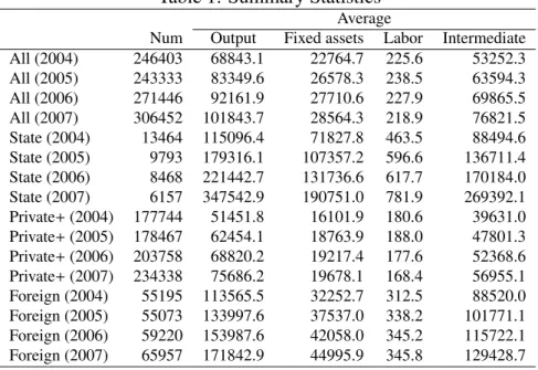
Table 1: Summary Statistics
Average
Num Output Fixed assets Labor Intermediate All (2004) 246403 68843.1 22764.7 225.6 53252.3 All (2005) 243333 83349.6 26578.3 238.5 63594.3 All (2006) 271446 92161.9 27710.6 227.9 69865.5 All (2007) 306452 101843.7 28564.3 218.9 76821.5 State (2004) 13464 115096.4 71827.8 463.5 88494.6 State (2005) 9793 179316.1 107357.2 596.6 136711.4 State (2006) 8468 221442.7 131736.6 617.7 170184.0 State (2007) 6157 347542.9 190751.0 781.9 269392.1 Private+ (2004) 177744 51451.8 16101.9 180.6 39631.0 Private+ (2005) 178467 62454.1 18763.9 188.0 47801.3 Private+ (2006) 203758 68820.2 19217.4 177.6 52368.6 Private+ (2007) 234338 75686.2 19678.1 168.4 56955.1 Foreign (2004) 55195 113565.5 32252.7 312.5 88520.0 Foreign (2005) 55073 133997.6 37537.0 338.2 101771.1 Foreign (2006) 59220 153987.6 42058.0 345.2 115722.1 Foreign (2007) 65957 171842.9 44995.9 345.8 129428.7
Table 1 reports summary statistics on the panel data by ownership sector.5) “State”
de-notes state-owned firms, including state-owned enterprises and solely state-funded corporations. “Private+” denotes domestic and non-state-owned firms, including collective-owned firms (and other hybrids) and privately funded enterprises. “Foreign” denotes firms with funds from Hong Kong, Macao, and Taiwan and those that are purely foreign-funded enterprises. The State sector shows the smallest number of firms and a sharp decrease of 54% from 2004 to 2007, whereas the number of private and foreign firms increased during the three years. The Private+ sector has the largest number of firms, accounting for 76% of the total in 2007. However, its output per firm is nearly five times smaller than that of state-owned firms in 2007, indicating that most private firms operate as small entities compared with state and foreign firms.
4.2
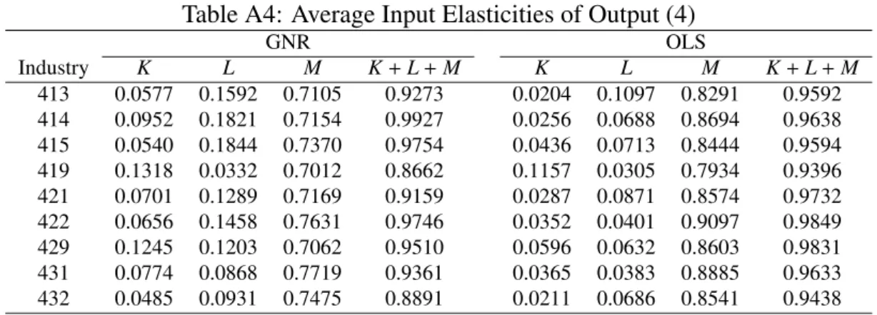
TFP and Output Elasticities
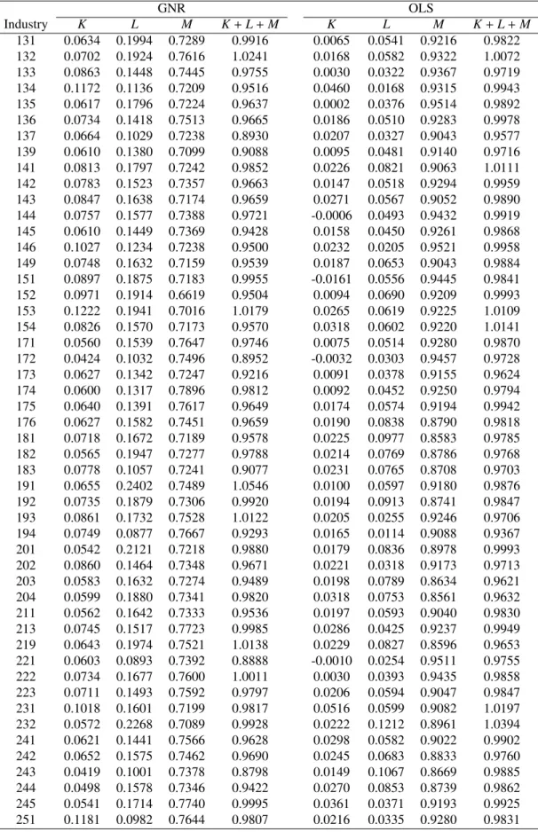
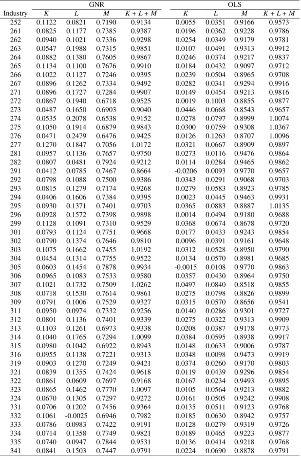
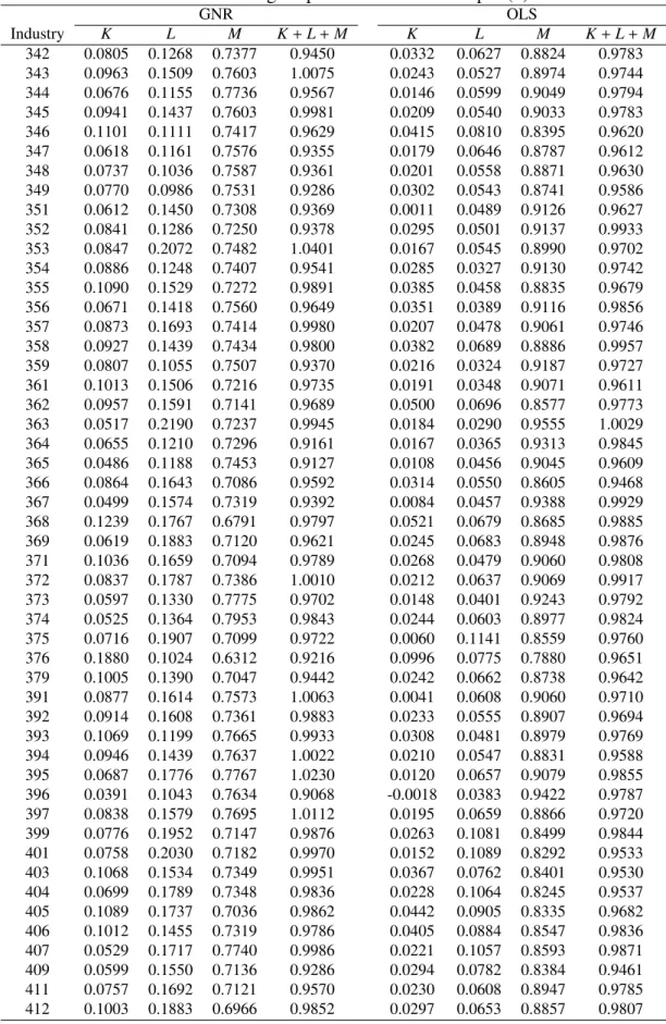
The production function in Equation (22) is separately estimated by industry using a three-digit industrial code.6) Appendix Tables A1–A4 report the estimates of the average output elastic-ities for each input and the sum of the elasticelastic-ities for capital, labor, and intermediate inputs. The estimates of GNR’s method are found to show lower average elasticities of intermediate inputs (ηM) than the OLS estimates in every industry. The difference between the GNR and
5)The tobacco industry is excluded from the database.
6)Tobacco (industrial codes 161, 162, and 169), and nuclear-related industries (253 and 424) are eliminated from
the sample. Industries 212, 214, 233, 402, and 423 are included in 211, 219, 232, 409, and 429, respectively. The estimation is implemented using R version 3.0.0 (R Development Core Team, 2009).
OLS estimates ofηM is 0.155 on average, and the OLS estimates are approximately 1.21 times
higher on average than the GNR estimates. These results are clearly expected and consistent with the estimation results in GNR (2013). The failure to control the endogenous bias from the correlation between flexible variables and unobservable productivity (ωit) is known to lead to
overestimates of the coefficients on flexible variables because positive productivity shocks are likely to increase the use of flexible inputs. The average elasticities of capital and labor as esti-mated by OLS are lower than the estimates based on the GNR method, which is also consistent with the empirical results in GNR (2013).
China’s intermediate input elasticities shown in Appendix Tables A1–A4 are higher than Colombia’s and Chile’s as estimated by GNR (2013). The data used in GNR (2013) are based on five three-digit manufacturing industries, and their estimates of input elasticities for these industries are 0.71 (Food Products), 0.56 (Textiles), 0.53 (Apparel), 0.53 (Wood Products), and 0.54 (Fabricated Metal Products) for Colombia, and 0.69, 057, 0.58, 0.62, and 0.53 for Chile, respectively. Compared with this paper’s estimates of the nearly corresponding industries (131, 171, 181, 203, and 341), Colombia’s and Chile’s estimates are lower in every case, indicating that China’s manufacturing production depends more on intermediate inputs.
5
Allocation E
fficiency
This section presents the results of the augmented OP and dynamic OP (AOP and ADOP) de-composition using China’s manufacturing firm-level productivity. These methods enable us to simultaneously quantify allocation efficiency within a group and between groups. The defini-tion of group j is required for this analysis. Secdefini-tion 5.1 shows the results based on the group defined as having 159 three-digit industrial sectors ( j = 1, 2, . . . , J; J = 159), and Section 5.2 reports the results based on the group defined as having three ownership sectors ( j = State, Private+, Foreign; J = 3).
5.1
Allocation E
fficiency of 3-digit Industrial Sectors
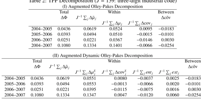
Table 2 reports the results of the AOP and ADOP decomposition based on the group of three-digit industrial sectors (J = 159). The change rate of the aggregate log TFP from 2004 to 2007 is 10.80%, and its annual average is 2.70%. Annual TFP growth rates tend to decrease annu-ally, such as 4.36% for 2004–05, 3.93% for 2005–06, and 2.51% for 2006–07. These figures are smaller than those estimated by Brandt, et al (2012), who showed that the annual average growth of aggregate TFP is 2.85% for a gross output production function from 1998 to 2007 (Brandt, et al., 2012, Table 2). However, the sample periods and estimation methods of this pa-per differ from their paper, and these results indicate the possibility that China’s manufacturing TFP growth tended to slow after 2004.
The ADOP decomposition reveals that new entering firms during 2004–2007 decreased aggregate manufacturing TFP by −1.20% points, whereas exiting firms increased it by 0.6% points. In the case of Slovenian manufacturing, the contribution of entering and exiting firms during 1995–2000 was 0.21% and 2.79% points, respectively (Melitz and Polanec, 2015). The contribution of China’s exiting firms on productivity is positive; however, the magnitude is much smaller than that in Slovenia’s case. These results indicate that entering firms in China are less efficient than surviving firms, whereas the exiting firms are slightly more inefficient
Table 2: TFP Decomposition (J = 159: three-digit industrial code)
(I) Augmented Olley-Pakes Decomposition
Total Within Between ∆Φ J−1∑j∆˜µj ∆ ˜cov J−1∑j∆µj J−1∑j∆covj 2004–2005 0.0436 0.0619 0.0524 0.0095 −0.0183 2005–2006 0.0393 0.0494 0.0510 −0.0015 −0.0101 2006–2007 0.0251 0.0221 0.0367 −0.0146 0.0030 2004–2007 0.1080 0.1334 0.1401 −0.0066 −0.0254
(II) Augmented Dynamic Olley-Pakes Decomposition
Total Within Between
∆Φ J−1∑j∆˜µj ∆ ˜cov J−1∑j∆µSj J−1 ∑ j∆covSj J−1 ∑ jentj J−1 ∑ jextj 2004–2005 0.0436 0.0619 0.0551 0.0080 −0.0037 0.0025 −0.0183 2005–2006 0.0393 0.0494 0.0553 −0.0013 −0.0066 0.0020 −0.0101 2006–2007 0.0251 0.0221 0.0395 −0.0115 −0.0075 0.0016 0.0030 2004–2007 0.1080 0.1334 0.1347 0.0047 −0.0120 0.0060 −0.0254
than are surviving firms. However, the average productivity gap between exiting and surviving firms is quite small, compared with Slovenia’s case. The entry and exit of manufacturing firms does not seem to contribute to the increase in aggregate TFP growth in China.
The contribution of allocation efficiency between groups (∆ ˜cov) to the aggregate manu-facturing TFP growth is −0.0254 for 2004–2007. If ∆ ˜cov was zero during 2004–2007, the aggregate log TFP change rate (∆Φ) would increase to 13.34% in Panel (I) and 13.47% in Panel (II), and these annual averages would be 3.34% and 3.37%, respectively. These results indi-cate that resource allocation among three-digit industrial sectors tends to worsen during this period, although the annual change rates increase over time. In contrast, the changes in the average allocation efficiency within each group are −0.0066 (AOP decomposition) and 0.0047 (ADOP decomposition), which indicate opposite signs for AOP and ADOP and small magni-tudes. The changes in allocation efficiency between the groups are found to affect the aggregate TFP changes more than those of the within-group allocation efficiency. The increase in misal-location between industrial sectors reduces aggregate TFP growth during 2004–2007 by annual average of 0.635% points.
Because the within allocation efficiency shown in Table 2 is the average of 159 three-digit sectors, the magnitude of the within effect for each sector is likely to vary among sectors. Fig-ure 1 shows a histogram of AOP and ADOP’s covariance terms within each sector (∆covj and
∆covS
j), which indicates that not all industries have negative values. However, the range is
from approximately 0.20 to −0.25 (without industry 379), and the number of sectors having positive values is 87 industries for the AOP decomposition and 99 industries for the ADOP decomposition. Furthermore, Panel (III) in the figure indicates a gap between the AOP and ADOP covariance terms. Considering the meaning of this gap is useful. AOP’s covariance change includes the contributions of both surviving firms and exiting-entering firms to the de-gree of allocation efficiency. In contrast, for ADOP, the focus is only on the change in allocation efficiency among surviving firms. Consequently, the difference in ∆covj − ∆covSj implies the
contributions of exiting firms and entering firms to the change in the allocation efficiency within sector j. A positive gap leads to the interpretation that exiting and/or entering firms contribute
(I) AOP −0.6 −0.4 −0.2 0.0 0.2 0 20 40 60 80 (II) ADOP −0.6 −0.4 −0.2 0.0 0.2 0 20 40 60 80
(III) AOP − ADOP
−0.2 −0.1 0.0 0.1 0.2 0 20 40 60 80
Figure 1: Allocation efficiency within each industrial sector.
Notes: The vertical axis represents the number of three-digit industrial sectors. The horizontal
axis is defined as∆covjfor panel (I),∆covSj for panel (II), and∆covj− ∆covSj for panel (III).
to improving allocation efficiency. As shown in Panel (III) of Figure 1, the gap differs among sectors and ranges from−0.16 to 0.21. The average is −0.011, and 107 of 159 sectors (67%) are plotted in the negative area, indicating that a firm’s entry to and/or exit from the market does not necessarily contribute to improving China’s manufacturing allocation efficiency.
What causes the difference in the within allocation efficiency (∆covj and ∆covSj) among
industrial sectors? Chen, et al. (2011) argued that the changes in China’s allocation efficiency have a negative relationship with the capital-labor ratio and the market shares of state-owned firms. Brandt et al. (2013) found that the misallocation of capital between state and non-state sectors tended to increase after 1997. These findings indicate that misallocation is expected to increase in relatively capital intensive industries, and/or in industries dominated by state-owned firms. Furthermore, it is possible that the spatial concentration of industries contributes to improving allocation efficiency because spatial concentration is likely to enhance competition among firms. Thus, less-productive firms are expected to exit the market and, consequently, production resources are allocated to more productive firms.
To explore the factors that change the variations in allocation efficiency, a regression analysis is conducted, using three-digit industrial sectors. The explained variables are the changes of within-allocation efficiencies (∆covj and∆covSj) during 2004–2007. The explanatory variables
are market share by ownership (State, Private+, and Foreign), aggregate industry-level capital-labor ratio, and the Ellison-Glaeser (EG) industry-concentration index (Ellison and Glaeser, 1997). The market shares are measured using gross output, and the EG index is based on county-level regions and the number of firm-level employees, such as:
EGj = ∑M m=1(sjm− s∗m)2− ( 1−∑m=1M s2 ∗m ) Hj ( 1−∑Mm=1s2 ∗m ) ( 1− Hj ) , (32)
where i, j, and m denote firm, industry, and county, respectively, and: sjm= xjm ∑M m=1xjm , s∗m = ∑J j=1xjm ∑J j=1 ∑M m=1xjm , Hj = Nj ∑ i∈ j ( xi∈ j ∑ i∈ jxi∈ j )2 ,
where x is the number of employees. All explanatory variables are based on observations in 2004.
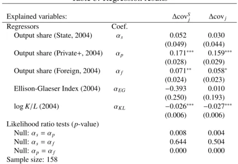
Table 3: Regression results
Explained variables: ∆covS
j ∆covj
Regressors Coef.
Output share (State, 2004) αs 0.052 0.030
(0.049) (0.044) Output share (Private+, 2004) αp 0.171∗∗∗ 0.159∗∗∗
(0.028) (0.029) Output share (Foreign, 2004) αf 0.071∗∗ 0.058∗
(0.024) (0.023) Ellison-Glaeser Index (2004) αEG −0.393 0.010
(0.250) (0.193) log K/L (2004) αKL −0.026∗∗∗ −0.027∗∗∗
(0.006) (0.006) Likelihood ratio tests (p-value)
Null:αs= αp 0.008 0.004
Null:αs= αf 0.644 0.504
Null:αp= αf 0.000 0.000
Sample size: 158
Notes: The sample is based on the number of three-digit industrial sectors,
except sector #379. Asterisks ***, **, and * indicate significant levels at 0.1%, 1%, and 5%, respectively.
Table 3 reports the regression results.7) The market shares of private and foreign firms have positive and significant coefficients, while the market share of state-owned firms is insignificant. The log K/L has a significantly negative relationship with changes in allocation efficiency. The coefficients of EG index show negative values that are not significant for ∆covSj and ∆covj.
Contrary to expectations, the spatial concentration of industries does not have a positive effect on the improvement in allocation efficiency. These results indicate that changes in allocation efficiency tend to improve in industries with private firms having higher market shares, and/or in relatively labor intensive industries.
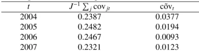
Exploring the magnitude of the allocation efficiency level is also useful. Table 4 provides the level of covariance terms within an industry and between industries. A comparison of panels (I) and (II) shows a small difference and the same tendency. Industry averages of the within-industry covariance terms fall between 0.22–0.24. These figures are not very small compared with those of other countries. According to Bartelsman et al. (2013; Table 1), the covari-ance term averages during 1993–2001 for eight countries were 0.51 (United States), 0.15 (UK), 0.28 (Germany), 0.24 (France), 0.30 (Netherlands), 0.16 (Hungary), -0.03 (Romania), and 0.04 (Slovenia). China’s manufacturing sector is at the same level as Germany’s. However, the
7)Because the sector #397 has negative extreme values for∆covS
j and∆covj, as shown in Figure 1, the sector is
between-industry covariance terms are very low, indicating negative values for several years and implying that improving the allocation efficiency between industries can make a significant contribution to increasing aggregate manufacturing TFP growth.
Table 4: Level of the covariance terms (J = 159)
(I) Augmented OP decomposition
t J−1∑jcovjt cov˜ t
2004 0.2387 0.0377 2005 0.2482 0.0194 2006 0.2467 0.0093 2007 0.2321 0.0123 (II) Augmented MP decomposition
J−1∑jcovS jt cov˜ S t t= 1 t = 2 t= 1 t= 2 t= 1 t= 2 2004 2005 0.2324 0.2404 0.0377 0.0194 2005 2006 0.2421 0.2408 0.0194 0.0093 2006 2007 0.2368 0.2253 0.0093 0.0123 2004 2007 0.2269 0.2316 0.0377 0.0123
In summary, allocation efficiency between industries worsened during 2004–2007, and a variation existed in the changes of within-industry allocation efficiency among industrial sec-tors. The within-allocation efficiency worsened for the sectors that use more capital and have firms with relatively higher state-owned market shares. These findings are consistent with those of Chen, et al. (2011) and Brandt, et al. (2013).
5.2
Allocation E
fficiency of Ownership Groups by Industrial Sector
The previous section showed the degree of allocation efficiency within each industrial sector and between industrial sectors. This section focuses on the allocation efficiency of ownership groups by three-digit industrial sector. The ownership groups are defined as j ∈ {State (S ), Private+ (P), and Foreign (F) sectors} (J = 3). Section 4 provides a definition of each sector. The author examines the extent of allocation efficiency within each ownership group and between groups using the three-digit industrial sector, and the following ADOP decomposition equation:
∆Φ(i) = 1 3 ∑ j∈{S,P,F} [ ∆µS j(i)+ ∆cov S
j(i)+ entj(i)+ extj(i)
]
+ ∆ ˜cov(i).
Note that i denotes a three-digit industrial sector in this section and the ADOP decomposition applies separately for each i = 1, 2, . . . , I∗. Because the three-digit industrial classification is relatively narrow, several industries have few or no firms in any of the three ownership sectors. To focus on the industries in which the three ownership sectors coexist, this analysis is con-ducted on the three-digit industrial sectors with more than 50 firms for each ownership sector. As a result, I∗ = 75 industrial sectors are used in this section.
5.2.1 Allocation Efficiency between Ownership Groups
Figure 2 presents the allocation efficiency between three ownership groups (∆ ˜cov(i)) during 2004–2007. Panel (A) of Figure 2 exhibits the plots of aggregate productivity changes ∆Φ(i),
−0.2 0.0 0.1 0.2 0.3 0.4 −0.10 −0.05 0.00 0.05 Changes of Productivity Changes of Co v ar iance (Betw een groups) 131 132 133 135 136 139 141 146 149 152 153 154 171 175 176 181 201 202 211 222 223231 232 251 261 262 263 264 266 267 272 274 303 311 312 313 314 315 316 319 323 331 335 341 342 343 351 352 353 354 355 357 358 359 361 362 363 366 367 368 369 371 372 375 376 391 392 393 401 405 406 411 412 421 429 −0.2 −0.1 0.0 0.1 0.2 −0.15 −0.10 −0.05 0.00 0.05
Changes of Productivity (State)
Changes of Mar k et share (State) 131 132 133 135 136 139 141 146 149 152 153 154 171 175 176 181 201 202 211 222 223 231 232 251 261 262 263 264 266 267 272 274 303 311 312 313 314 315 316319 323 331335 341 342 343 351 352 353 354 355 357 358 359 361 362 363 366 367 368 369 371 372 375 376 391 392 393 401 405 406 411 412 421 429
(A) Plots of∆Φ (horizontal axis) and ∆ ˜cov (vertical axis) (B) Decomposition of∆ ˜cov (State)
−0.10 0.00 0.05 0.10 0.15 −0.05 0.00 0.05 0.10 0.15
Changes of Productivity (Private+)
Changes of Mar k et share (Pr iv ate+) 131 132 133 135 136 139 141 146 149 152 153 154 171 175 176 181 201 202 211 222 223 231 232 251 261 262 263 264 266 267 272 274 303 311 312 313314 315 316 319 323 331 335 341 342 343 351 352 353 354 355358 359 357 361 362 363 366 367 368 369 371 372 375 376 391 392 393 401 405 406 411 412 421 429 −0.15 −0.05 0.00 0.05 0.10 −0.15 −0.05 0.05 0.10
Changes of Productivity (Foreign)
Changes of Mar k et share (F oreign) 131 132 133 135 136 139 141 146 149 152 153 154171 175 176 181 201 202 211 222 223 231 232 251 261 262 263 264 266 267 272 274 303 311 312 313 314 315 316 319 323 331 335 341 342 343 351 352 353 354 355 357358 359 361 362 363 366 367 368 369 371 372 375 376 391 392 393 401 405 406 411 412 421 429
(C) Decomposition of∆ ˜cov (Private+) (D) Decomposition of∆ ˜cov (Foreign)
Figure 2: Changes in allocation efficiency between ownership groups during 2004–2007
Notes: Red-colored plots denote industries with positive∆ ˜cov values in Panel (A), whereas blue-colored plots denote industries with negative∆ ˜cov values.
and the changes in allocation efficiency between the three ownership groups, ∆ ˜cov(i). Al-though the average of∆ ˜cov(i) is almost zero (−0.007), it varies among industries, ranging from −0.114 to 0.09. In all, 30 industrial sectors are plotted in the positive area of the vertical axis (∆ ˜cov(i) > 0), indicating that these industries tend to improve resource allocation among the three ownership groups.
To investigate the source of the variation in∆ ˜cov(i), it is rewritten as follows (suppress i to ease notation): ∆ ˜cov= ∑ j∈{S,P,F} (xj2yj2− xj1yj1) = ∑ j∈{S,P,F} (yj2∆xj2+ xj1∆yj2) (33) where xjt = wjt− 1/J ∑ jwjtand yjt = ˜µjt− 1/J ∑
jµ˜jtfor t = 1, 2. ∆xjtand∆yjtdenote changes
in the demeaned aggregate productivity and market share for each ownership sector during 2004–2007. The relationship among the three variables (∆ ˜cov, ∆xjt, and ∆yjt) is plotted in
Panels (B)–(D) of Figure 2 by ownership. The red-colored plots denote industries with positive ∆ ˜cov values in Panel (A), whereas the blue-colored plots denote industries with negative∆ ˜cov values.8)
As shown in Panel (B), the State sector’s market shares decreased in most industrial sectors, and red plots in Panel (B) are primarily distributed in the third quadrant. This result indicates that resource allocation between ownership groups (∆ ˜cov) tends to improve in industries in which the State sector’s market share and productivity both decrease. In contrast, the blue plots in Panel B are primarily distributed in the fourth quadrant, indicating that the resource allocation between ownership groups are likely to worsen in industries in which the State sector’s market share decreases but productivity increases.
Panel (C) shows the relationship between the changes in the Private+ sector’s market share and productivity. Contrary to Panel (B), the red and blue plots are primarily distributed in the first and second quadrants, respectively, indicating that the resource allocation between ownership groups tends to improve in industries in which the Private+ sector’s market share and productivity both increase and worsen in industries in which the Private+ sector’s market share increases but productivity decreases. In contrast, the Foreign sector (Panel (D)) does not show a clear relationship between red and blue plots.
In summary, the allocation efficiency between ownership sectors tends to improve in in-dustries in which the market share moves from the less-productive State sector to the more-productive Private+ sector. In contrast, the allocation efficiency tends to worsen in industries in which 1) the State sector’s productivity relatively increases despite a decrease in its market share or 2) the Private+ sector’s productivity does not grow compared with the other sectors despite an increase in its market share.
5.2.2 Within-Effects for Each Ownership Group
Figure 3 reports the histograms of the within-effects. The vertical axis defines the number of three-digit industrial sectors (i = 1, 2, . . . , 75). Panels (A), (B) and (C) show allocation
8)Note that the first and third quadrants in Panels (B)–(D) indicate the positive relationship between the changes
in market share and productivity. However, this positive relationship does not necessarily produce positive∆ ˜cov values. As is clear from Equation (33),∆ ˜cov does not necessarily become positive even if the sign of∆xj2is the
State −0.4 −0.2 0.0 0.1 0.2 0.3 0 10 20 30 40 Private+ −0.2 −0.1 0.0 0.1 0.2 0 10 20 30 40 Foreign −0.2 −0.1 0.0 0.1 0 10 20 30 40
(A) Allocation efficiency within a group j (∆covSj(i), j=State, Private+, Foreign)
State −0.10 0.00 0.10 0.20 0 10 20 30 40 Private+ −0.06 −0.02 0.02 0.06 0 10 20 30 40 Foreign −0.04 0.00 0.04 0.08 0 10 20 30 40
(B) Entry effects within a group j (entSj(i), j=State, Private+, Foreign)
State −0.1 0.0 0.1 0.2 0.3 0 10 20 30 40 50 60 Private+ −0.04 0.00 0.04 0.08 0 10 20 30 40 50 60 Foreign −0.15 −0.05 0.05 0.10 0 10 20 30 40 50 60
(C) Exit effects within a group j (extSj(i), j=State, Private+, Foreign) Figure 3: Decomposition of the within-effect by ownership during 2004–2007
Notes: The vertical axis shows the number of three-digit industrial sectors (i =
efficiency ∆covS
j(i), entry effects ent S
j(i), and exit effects ext S
j(i) within a group j ∈ {S, P, F},
respectively.
Panel (A) shows that the means of these histograms is −0.007 (State), 0.020 (Private+), and −0.007 (Foreign), and that the shares of the number of sectors with ∆covS
j(i) > 0 are
46.7%, 76.0%, and 56%, respectively. Although the values of ∆covSj(i) are distributed broadly for each group, the Private+ group tends to improve its allocation efficiency among firms dur-ing 2004–2007. The entry effect in Panel (B) shows that the means for each group are 0.019 (State), −0.14 (Private+), and −0.007 (Foreign), and the shares of the number of sectors with
entS
j(i) > 0 are 48.0%, 21.3%, and 29.3%, respectively. This result indicates that new entry
firms in the Private+ and Foreign groups during 2004–2007 have, on average, lower productiv-ity than existing firms for each group. Consequently, they have a negative effect on aggregate productivity growth. Furthermore, the exit effect of the Private+ group shown in Panel (C) is also small. The means are 0.026 (State), 0.0019 (Private+), and 0.003 (Foreign), and the shares of the number of sectors with extSj(i)> 0 are 85.3%, 53.3%, and 85.3%, respectively, implying that relatively nonproductive firms in the Private+ group are not likely to exit the market.
In summary, the Private+ sector tends to have more industrial sectors improving allocation efficiency among firms, compared with State and Foreign sectors. However, the entry and exit effects for Private+ are very weak. In particular, the entry effect has negative values for many industrial sectors, indicating that new firms in the Private+ sector tend to be less productive than existing firms and drive down aggregate productivity growth.
6
Conclusions
Are changes in resource allocation important to driving the growth of aggregate TFP? Answer-ing this question requires a quantitative measure of allocation efficiency. This paper provides a new measure of allocation efficiency that is an extension of the productivity decomposition methods proposed by Olley and Pakes (1996) and Melitz and Polanec (2015). This new measure enables us to simultaneously capture the degree of misallocation within a group and between groups, and parallel to capturing the contribution of entering and exiting firms to aggregate TFP growth. Because the methods used by Olley and Pakes (1996) and Melitz and Polanec (2015) cannot capture the degree of allocation efficiency between groups, this new measure can be considered a group-wise extension of their methods.
The measure of allocation efficiency is applied to China’s manufacturing firm-level data from 2004 to 2007. This paper uses two definitions of groups: (1) 159 industrial groups based on a three-digit industrial classification and (2) three ownership groups (State, Private+, For-eign sectors). Firm-level productivity used to calculate productivity decomposition is estimated using a structural estimation method proposed by Gandhi et al. (2013). The main findings of this paper are summarized as follows:
1. New entering and exiting firms did not contribute significantly to the increase in growth of aggregate manufacturing TFP.
2. Misallocation between 159 industrial sectors tended to increase during 2004–2007, which reduced aggregate TFP growth during 2004–2007 by an annual average of 0.635% points. The changes in allocation efficiency within each industrial sector during 2004–2007 var-ied widely among sectors. However its average is almost zero, indicating that the within-effects do not significantly affect aggregate TFP growth.
3. Misallocation within an industrial sector was found to increase for sectors using more capital and having firms with relatively higher state-owned market shares. These findings are consistent with those of Chen, et al. (2011) and Brandt, et al. (2013).
4. Misallocation between three ownership groups declined in 30 of the 75 three-digit indus-trial sectors, indicating that these industries improved resource allocation among the three ownership groups. Furthermore, misallocation tended to decline in industries wherein market shares move from the less-productive State sector to the more-productive Pri-vate+ sector. In contrast, misallocation tended to worsen in industries in which 1) the State sector’s productivity relatively increases despite decreases in its market share or 2) the Private+ sector’s productivity does not grow compared with that of the other sectors despite increases in its market share.
5. The Private+ sector has more industrial sectors improving the within-allocation efficiency among firms compared with the State and Foreign sectors. However, the entry and exit effects for the Private+ sector were very small. In particular, the entry effect has negative values for many industrial sectors, indicating that new firms in the Private+ sector tended to be less productive than existing firms, driving down aggregate productivity growth. These empirical results lead us to conclude that misallocation in China’s manufacturing sec-tor tended to increase during 2004–2007 that, particularly the increase in misallocation between industrial sectors had a significant negative effect on aggregate TFP growth. Furthermore, al-location efficiency tended to improve in industrial sectors in which 1) the production process is not capital intensive and 2) non-state-owned firms are relatively productive and have higher market share than state-owned firms.
What is behind the behavior of allocation efficiency in China? According to previous stud-ies, financial frictions are believed to be an important source of misallocation (Caggese and Cu˜nat, 2013; Midrigan and Xu, 2014). The increase in misallocation in China could be at-tributed to unequal access to factor resources, such as capital from bank loans, subsidies, and land, between state-owned and non-state owned firms. Since the 2000s, one debate has been over the state sector’s advantageous access to capital resources compared with the private sector, a phenomenon called Guojin Mintui (i.e., the state advances, the private sector retreats). Such a favorable environment for the state sector may impede the growth of the private sector, causing resource allocation to deteriorate. In addition, as Brandt et al. (2013) argued, regional policies such as Xibu Kaifa (i.e., develop the great west) may be related to the increase in misallocation. If the government promotes the reallocation of investment resources toward less-productive sectors, doing so should worsen resource allocation.
Identifying the source of misallocation is challenging, but misallocation worsened in China’s manufacturing sector during 2004–2007, in accordance with the findings of this paper. There-fore, reexamining the regional development policies and the equity of competitive conditions among firms in the financial market in terms of optimal resource allocation is crucially impor-tant.
Finally, the difference should be noted between the two measures for allocation efficiency: 1) the covariance type, originally developed by Olley and Pakes (1996), and 2) the dispersion type, discussed by Hsieh and Klenow (2009). The former assesses the degree of allocation ef-ficiency using the relationship between market share and productivity, whereas the latter uses the degree of dispersion (e.g., standard deviations) of firm-level productivity within a sector
as the measure of allocation efficiency. A higher covariance measure indicates more-efficient resource allocation, whereas a lower dispersion measure indicates more-efficient resource al-location. However, these two measure are likely to provide inconsistent results because the decrease in the dispersion might lead to a decline in the covariance. What are the main sources of this inconsistency? Although this issue is beyond the scope of this paper, it must be resolved.
References
Ackerberg, D. A., K. Caves, and G. Frazer. (2006) “Structural identification of production function.” Unpublished Manuscript, UCLA Economics Department.
Bartelsman, E., J. Haltiwanger, and S. Scarpetta. (2013) “Cross-country differences in produc-tivity: the role of allocation and selection.” American Economic Review, 103(1): 305–334. Bond, S. and M. S¨oderbom. (2005) “Adjustment costs and the identification of Cobb Douglas
production Functions.” mimeo.
Brandt, L., J. Van Biesebroeck, and Y. Zhang. (2012) “Creative accounting or creative destruc-tion? Firm-level productivity growth in Chinese manufacturing.” Journal of Development
Economics, 97(2): 339–351.
Brandt, L., T. Tombe, and X. Zhu. (2013) “Factor market distortions across time, space and sectors.” Review of Economic Dynamics, 16(1): 39–58.
Caggese, A. and V. Cu˜nat. (2013) “Financing constraints, firm dynamics, export decisions, and aggregate productivity.” Review of Economic Dynamics, 16(1): 177–193.
Chen, S., G. H. Jefferson, and J. Zhang. (2011) “Structural change, productivity growth and industrial transformation in China.” China Economic Review, 22(1): 133–150.
Chenery, Hollis, Sherman Robinson, Moshe Syrquin. (1986) Industrialization and Growth: A
Comparative Study. New York: Published for the World Bank by Oxford University Press.
Collard-Wexler, A. and J. De Loecker. (2015) “Reallocation and technology: evidence from the U.S. steel industry.” American Economic Review, forthcoming.
Gandhi, A., S. Navarro, D. Rivers. (2013) “On the identification of production functions: how heterogeneous is productivity?” mimeo.
Ellison, G., and E. L. Glaeser. (1997) “Geographic concentration in U.S. manufacturing indus-tries: a dartboard approach.” Journal of Political Economy, 105(5): 889–927.
Herrendorf, B., R. Rogerson, and ´A. Valentinyi. (2013) “Growth and structural transformation.”
NBER Working Paper, No. 18996.
Hsieh, C. and P. J. Klenow. (2009) “Misallocation and manufacturing TFP in China and India.”
Quarterly Journal of Economics, 124(4): 1403–1448.
Kuznets, S. (1979) “Growth and Structural Shifts.” in Economic Growth and Structural Change
in Taiwan, edited by Walter Galenson, 15–131. Ithaca and London: Cornell University
Press.
Levinsohn, J. and A. Petrin. (2003) “Estimating production functions using inputs to control for unobservables.” Review of Economic Studies, 70(2): 317–341.
Marschak, J. and W. H. Andrews. (1944) “Random simultaneous equations and the theory of production ” Econometrica, 12(3-4): 143–205.
Melitz, M. J. and S. Polanec. (2015) “Dynamic Olley-Pakes productivity decomposition with entry and exit.” RAND Journal of Economics, 46(2): 362–375.