分数階微分方程式のリー環対称性による研究

分数階微分方程式のリー環対称性による研究

ドルジゴトフ, ホンゴズル

https://doi.org/10.15017/1931728

出版情報：Kyushu University, 2017, 博士（数理学）, 課程博士 バージョン：

権利関係：

fractional differential equations

Khongorzul Dorjgotov

Supervisor: Prof. H. Ochiai

Graduate School of Mathematics Kyushu University

This dissertation is submitted for the degree of Doctor of Philosophy

February 2018

I would like to express my sincere gratitude to my supervisor Prof. Hiroyuki Ochiai for the earnest hearing to my boring talks and giving me the turning point-comments and insightful remarks, and for being considerate to my family. I could not have imagined having a better advisor for my Ph.D study.

I also thank my lifetime partner and colleague Uuganbayar Zunderiya for everything.

Without you, this work would not be possible.

Last but not least, I would like to thank my parents for being always on my side and giving continuous encouragement, and to my little son for taking care of himself and being a good boy when mommy was working.

We study time fractional linear and nonlinear evolution systems with variable coefficients via Lie symmetry analysis. For both classes of the system, we give complete group classification and for linear time fractional evolutions systems, we give exact solutions corresponding to infinitesimal symmetries of optimal systems of Lie algebras generated by infinitesimal symmetries. For fractional nonlinear evolution system, we give explicit invariant solutions in some particular cases. The group invariant solutions are expressed in terms of special functions. More concretely, with the help of the infinitesimal symmetries we reduce the system of time fractional partial differential equations into a system of fractional ordinary differential equations which have Euler-type integer order differential operator up to second order. Even though finding exact solutions to fractional differential equations is not easy, we are able to give solutions to fractional differential equations with Euler-type integer order differential operator up to arbitrary high order.

List of figures ix

List of tables xi

1 Introduction 3

1.1 Fractional derivative . . . 3

1.1.1 Definitions of fractional derivatives . . . 3

1.1.2 Fractional derivative of power functions . . . 6

1.1.3 Elementary properties of fractional derivative . . . 6

1.2 Special functions . . . 8

1.3 Basics of Lie symmetry analysis for differential equations . . . 12

1.3.1 Main concepts of Lie symmetry analysis of PDE . . . 12

1.3.2 Lie symmetry analysis of FPDE . . . 16

1.3.3 Lie symmetry analysis of the system of FPDE . . . 18

2 Solutions of linear fractional differential equations 23 2.1 Construction of exact solutions . . . 24

2.1.1 Solutions expressed in terms of Mittag-Leffler functions . . . 24

2.1.2 Solutions expressed in terms of generalized Wright functions . . 26

2.1.3 Solutions expressed in terms of Fox H-functions . . . 32

2.2 Solutions of FODE with higher order derivatives . . . 39

3 Lie symmetry analysis of time fractional linear system 45 3.1 Classification of group invariant solutions . . . 46

3.1.1 Invariant solutions of (3.1) with c(x) =m₁(x+m₂)^m3 . . . 46

3.1.2 Invariant solutions of (3.1) with c(x) =m₁e^m2x . . . 50

3.1.3 Invariant solutions of (3.1) with c(x)≡c . . . 51

3.2 Some properties of the solutions . . . 54

3.3 Invariant solutions of the special case α= 1 . . . 58

3.3.1 Solutions of (3.1) with c(x) = x^m (m ̸= 0,1) and α= 1 . . . 59

3.3.2 Solutions of (3.1) with c(x) = x and α= 1 . . . 65

3.3.3 Solutions of (3.1) with c(x) = e^−x2 and α = 1 . . . 66

3.3.4 Solutions of (3.1) with c(x) = 1 and α= 1 . . . 67

4 Lie symmetry analysis of time fractional nonlinear system 69 4.1 Lie symmetry analysis of (4.1) . . . 70

4.2 Classification of invariant solutions of (4.1) . . . 73

4.2.1 Case 1. For arbitraryb(u),but b(u)̸=ku^m . . . 73

4.2.2 Case 2. b(u) =ku^m . . . 74

4.3 Invariant solutions of (4.1) . . . 79

4.3.1 Invariant solutions of (4.1) corresponding to U₁ . . . 80

4.3.2 Invariant solutions of (4.1) corresponding to U₄ in Case 2.1 . . . 80

4.3.3 Invariant solutions of (4.1) corresponding to U₅ in Case 2.1 . . . 81

4.3.4 Invariant solutions of (4.1) corresponding to U₂ in Case 2.2 . . . 82

4.3.5 Invariant solutions of (4.1) corresponding to U₄ in Case 2.2 . . . 83

References 85

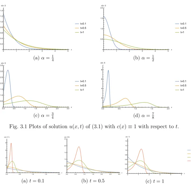
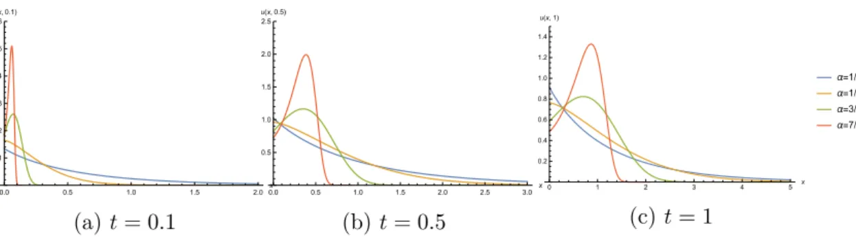
1.1 The Fox H-function contour . . . 10 3.1 Plots of solution u(x, t) of (3.1) withc(x)≡1 with respect to t. . . . . 57 3.2 Plots of solution u(x, t) of (3.1) with c(x) ≡ 1 for various order α of

fractional derivative. . . 57 3.3 Plots of solution u(x, t) of (3.1) withc(x) =x¹⁴ with respect tot. . . . . 58 3.4 Plots of solution u(x, t) of (3.1) with c(x) = x¹⁴ for various orderα of

fractional derivative. . . 58

3.1 Commutator table for case c(x)≡c.. . . 51

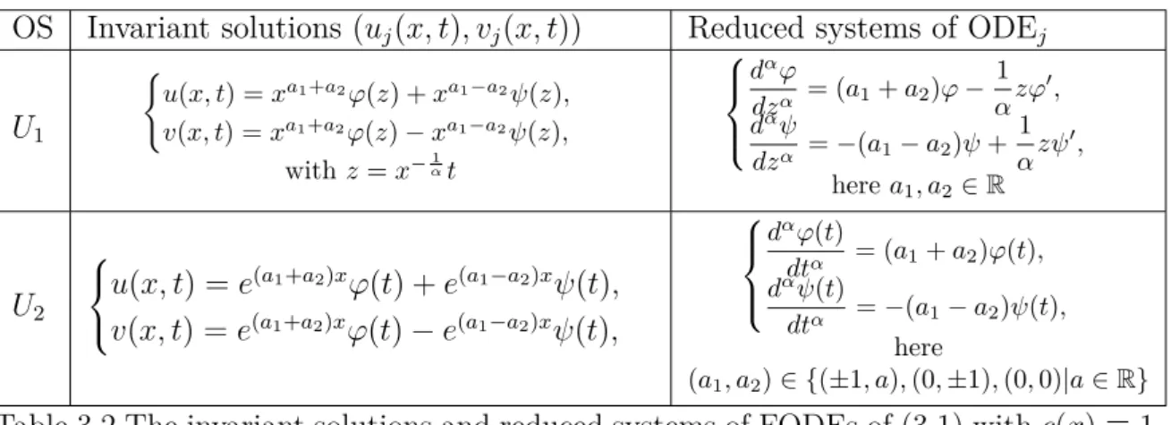
3.2 The invariant solutions and reduced systems of FODEs of (3.1) with c(x)≡1. . . 52

4.1 Commutator table for Case 1. . . 73

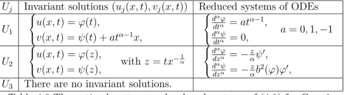
4.2 The optimal systems and reduced systems of (4.1) for Case 1 . . . 74

4.3 Commutator table for Case 2.1. . . 75

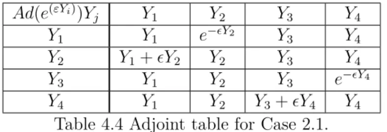
4.4 Adjoint table for Case 2.1. . . 75

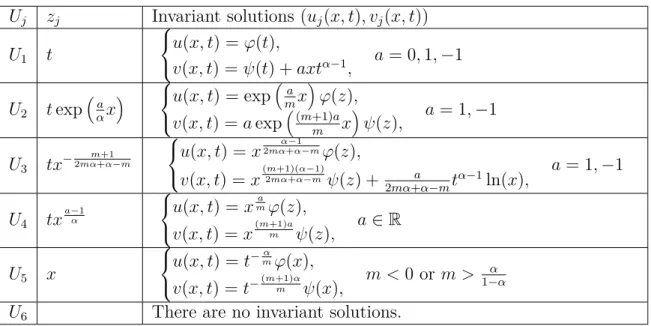
4.5 Similarity variables z_j and invariant solutions (u_j, v_j) for Case 2.1. . . . 76

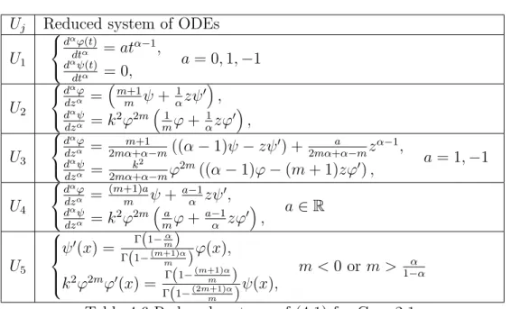
4.6 Reduced systems of (4.1) for Case 2.1. . . 77

4.7 Commutator table for Case 2.2. . . 77

4.8 Adjoint table for Case 2.2. . . 77

4.9 Similarity variables z_j and invariant solutions (u_j, v_j) for Case 2.2. . . . 78

4.10 Reduced systems of (4.1) for Case 2.2. . . 79

A symmetry of differential equation is a transformation that preserves the form of the equation. Although determining symmetries can be computationally intensive, Lie symmetry analysis is an efficient, algorithmic method for solving various types of differential equations. For example through Lie symmetry analysis, we can find invariant solutions to two dimensional partial differential equations by reducing them into the ordinary differential equations. Lie symmetry analysis is well developed for partial and ordinary differential equations. In last few decades, fractional differential equations have emerged in applications. The fractional derivatives are also known as integro-differential operators, and they characterize and model processes with long term memory rather than integer order derivatives which characterize local properties.

Gazizov R. K. et. al. [Vest. UGATU 9 3(21): 125-135 (2007)] presented formulas for extended infinitesimals of fractional ordinary and partial differential equations, and developed Lie symmetry analysis for fractional differential equations. Huang Q. et. al.

[J. Math. Phys. 56 123504 (2015)] first generalized Lie symmetry analysis of fractional differential equation into a system of fractional differential equations. Then, Singla K.

et. al. [J. Math. Phys. 57 101504 (2016)] tried to correct the formula for extended infinitesimals which were obtained in Huang’s work.

We study time fractional linear and nonlinear evolution systems with variable coefficients via Lie symmetry analysis. To study the fractional systems we have obtained formulas for extended infinitesimals that match with the ones obtained neither by Huang nor by Singla. The linear time fractional evolution systems of our interest were studied before by Huang. Huang obtained only elementary monomial solutions and determined that there are three types of functions for the variable coefficient of time fractional linear evolution systems, so that the fractional linear evolution system admits symmetries. Here, we not only give complete group classification of invariant solutions but also exact solutions corresponding to infinitesimal symmetries of optimal systems of Lie algebras of infinitesimal symmetries. The group invariant solutions are expressed in terms of three kinds of special functions: the Mittag-Leffler functions, the

generalized Wright functions and the Fox H-functions. Which of these special functions we use in any given case depends on order of the fractional derivative and right hand sides of the equations in the fractional linear system. For fractional nonlinear evolution system, we give complete group classification along with explicit invariant solutions in some particular cases.

In briefly, our method to study fractional evolution systems is as follows: We reduce the system of time fractional partial differential equations into a system of fractional ordinary differential equations with the help of the infinitesimal symmetries, which were obtained by solving the equation of invariance surface condition. Then, we obtain group invariant solutions to the original system by finding solutions to the reduced systems. The reduced systems of fractional linear evolution systems become systems of fractional differential equations with Euler-type integer order differential operator.

Even though finding exact solutions to fractional differential equations is not easy, we are able to give solutions to these reduced systems by showing some contiguity relations of special functions. More concretely, we reduce the problem of finding non-trivial solutions to Euler-type, linear fractional differential equations with higher order integer derivatives into a problem of finding roots of algebraic polynomials.

The linear and nonlinear fractional systems of our interest correspond to generalized time fractional diffusion-wave equations. In other words, for special values of order of fractional derivative the time fractional evolution systems correspond to the well-known diffusion or wave equations. Moreover, we show that the invariant solutions correspond to known solutions of diffusion and wave equations after applying some transformations.

Also, Buckwar E. et. al. [J. Math. Anal. Appl. 227(1998) etc.] studied time fractional diffusion-wave equations with constant coefficient via scaling symmetry and whenα is between 0 and 1, Metzler R. et. al. [Physica A 211 (1994)] gave solutions to time fractional diffusion-wave equations with variable coefficient using fractional Laplacian transformations. For particular values of parameters, the solutions that we obtained correspond to these solutions as well.

Introduction

1.1 Fractional derivative

Here we explain the derivatives of arbitrary real order, which unify and generalize the notions of integer order differentiation. Fractional derivatives provide an excellent instrument for the description of memory and hereditary properties of various materials and processes [24].

The following definitions and elementary properties are taken from [20]. The functions f(t) that we can take fractional derivatives are defined on the closed interval 0≤ t≤T, bounded everywhere in the half open interval 0 < t≤T and have better behavior at the lower limit 0 than has t⁻¹,which means:

limt→0tf(t) = 0.

We can also take fractional derivatives from so-called differintegrable series:

f(t) = t^p

∞

X

j=0

a_jt^nj, a₀ ̸= 0, p > −1, n∈Z+.

Notice that phas been chosen to ensure that the leading coefficient is nonzero. Most of the special functions of mathematical physics are differintegrable series according to this definition.

1.1.1 Definitions of fractional derivatives

In the literature, there exist many approaches and various definitions. But the most common ones are: the Grünwald-Letnikov derivative, the Caputo derivative and the

Riemann-Liouville derivative [24]. From here on, the value of n∈N0 ={0,1,2, . . .} is determined by

n−1< α < n.

The Grünwald-Letnikov derivative:

We know the higher order integer derivatives are determined as dⁿ

dtⁿf(t) = lim

h→0

1 hⁿ

n

X

k=0

(−1)^k n k

!

f(t−kh).

So, we generalize the order n to positive real α: d^α

dt^αGL

f(t) := lim

h→0

1 h^α

n

X

k=0

(−1)^k α k

!

f(t−kh)

=

n−1

X

k=0

f^(k)(0)t^k−α

Γ(k−α+ 1) + 1 Γ(n−α)

Z t 0

(t−τ)^n−α−1f⁽ⁿ⁾(τ)dτ, where f^(k)(t)∈C[0, t] fork = 1,2, . . . , n and

α k

!

= Γ(α+k) Γ(α) The Riemann-Liouville derivative:

d^α dt^αRL

f(t) :=







dⁿ

dtⁿf(t), for α=n ∈N,

1 Γ(n−α)

dⁿ dtⁿ

Rt

0(t−τ)^n−α−1f(τ)dτ, for α∈(n−1, n) with n∈N. (1.1) The Caputo derivative:

d^α dt^αC

f(t) := 1 Γ(n−α)

Z t 0

(t−τ)^n−α−1f⁽ⁿ⁾(τ)dτ.

These definitions correspond to each other in certain cases. We can see that if f^(k)(0) = 0 for k = 0, . . . , n−1 then the Grünwald-Letnikov derivative corresponds to the Caputo derivative. Also, if we take an assumption that the function f(t) isn times continuously differentiable, then integrating by parts and differentiating (1.1) we

come at the definition of Grünwald-Letnikov derivative:

d^α dt^αRL

f(t) = 1

Γ(n−α) dⁿ dtⁿ

Z t 0

f(τ)(t−τ)^n−α−1dτ

= 1

Γ(n−α+ 1) dⁿ dtⁿ

Z t 0

−f(τ)d(t−τ)^n−α

= 1

Γ(n−α+ 1) dⁿ dtⁿ



−f(τ)(t−τ)^n−α

t

0

+

Z t 0

f^′(τ)(t−τ)^n−αdτ





= f(0)

Γ(n−α+ 1) dⁿ

dtⁿt^n−α+ 1 Γ(n−α+ 1)

dⁿ dtⁿ

Z t 0

f^′(τ)(t−τ)^n−αdτ

= f(0)t^−α

Γ(1−α) + 1 Γ(n−α+ 1)

dⁿ dtⁿ

Z t 0

f^′(τ)(t−τ)^n−αdτ. (1.2) Interchanging the order of differentiation and integration [24]

d dt

Z t 0

F(t, τ)dτ =

Z t 0

∂F(t, τ)

∂t dτ +F(t, t−0) in (1.2), it equals to

d^α dt^αRL

f(t) = f(0)t^−α

Γ(1−α) + 1 Γ(n−α)

dⁿ⁻¹ dtⁿ⁻¹

Z t 0

f^′(τ)(t−τ)^n−α−1dτ

= f(0)t^−α

Γ(1−α) + f^′(0) Γ(n−α+ 1)

dⁿ⁻¹ dtⁿ⁻¹t^n−α

+ 1

Γ(n−α+ 1) dⁿ⁻¹ dtⁿ⁻¹

Z t 0

f^′(τ)(t−τ)^n−αdτ

= f(0)t^−α

Γ(1−α) +f^′(0)t^1−α

Γ(2−α) + 1 Γ(n−α)

dⁿ⁻² dtⁿ⁻²

Z t 0

f^′′(τ)(t−τ)^n−α−1dτ ...

=

n−1

X

k=0

f^(k)(0)t^k−α

Γ(k−α+ 1) + 1 Γ(n−α)

Z t 0

(t−τ)^n−α−1f⁽ⁿ⁾(τ)dτ

= d^α dt^αGL

f(t), since limτ→t−0(t−τ)^n−α = 0.

In this work, we adopt the Riemann-Liouville derivative d^α

dt^α ≡ d^α dt^αRL

.

A major difference between the Riemann-Liouville derivative and the Caputo derivative is that the Caputo derivative of a constant is 0,whereas the Riemann-Liouville derivative of a constant is non-zero, as will be seen in the next section.

1.1.2 Fractional derivative of power functions

Let us take fractional derivative of function t^p : d^α

dt^αt^p = 1 Γ(n−α)

dⁿ dtⁿ

Z t 0

(t−τ)^n−α−1τ^pdτ.

Substituting τ =tu into the above expression, we obtain d^α

dt^αt^p = 1 Γ(n−α)

dⁿ dtⁿ

Z 1 0

(t−tu)^n−α−1t^p+1u^pdu

= 1

Γ(n−α) dⁿ dtⁿ

t^{n−α−1+p+1}

Z 1 0

(1−u)^n−α−1u^pdu

. We can use the beta function formula for p >−1:

d^α

dt^αt^p = 1 Γ(n−α)

dⁿ dtⁿ

ht^n−α+pB(p+ 1, n−α)ⁱ

= dⁿ dtⁿ

t^n−α+p Γ(n−α)

Γ(p+ 1)Γ(n−α) Γ(n−α+p+ 1)

= Γ(p+ 1)

Γ(n−α+p+ 1) dⁿ

dtⁿt^n−α+p

= Γ(p+ 1)

Γ(p+ 1−α)t^p−α. (1.3)

As a corollary, for p= 0, we have a fractional derivative of the unit function:

d^α

dt^α1 = t^−α Γ(1−α), then for any constant function including zero, we have:

d^α

dt^αC=C t^−α Γ(1−α).

1.1.3 Elementary properties of fractional derivative

The following properties are useful in our calculation.

Linearity

The linearity of the fractional derivative follows directly from the definition:

d^α dt^α

N

X

j=0

C_jf_j(t) =

N

X

j=0

C_j d^α

dt^αf_j(t) for N ∈N. Taking derivative from a series

If the series ^Pf_j(t) as well as the series ^P_dt^dααf_j(t) converge uniformly in 0< t < T, then

d^α dt^α

∞

X

j=0

f_j(t) =

∞

X

j=0

d^α

dt^αf_j(t) for 0< t < T.

Scale change of the Riemann-Liouville derivative For β ∈R, we have the following property:

d^α

dt^αf(βt) = 1 Γ(n−α)

dⁿ dtⁿ

Z t 0

(t−τ)^n−α−1f(βτ)dτ

= 1

Γ(n−α) dⁿ dtⁿ

Z βt 0

t− T β

!n−α−1

f(T)1 βdT

= β^α−n Γ(n−α)

dⁿ dtⁿ

Z βt 0

(βt−T)^n−α−1f(T)dT

= β^α

Γ(n−α) dⁿ d(βt)ⁿ

Z βt 0

(βt−T)^n−α−1f(T)dT

= β^α d^α

d(βt)^αf(βt).

Generalized Leibniz’s rule

The fractional differentiation rule for product of two functions is d^α

dt^α(f(t)g(t)) =

∞

X

j=0

α j

!d^α−j

dt^α−jf(t)d^j

dt^jg(t). (1.4)

Composition rule or Sequential derivative

∂^α

∂t^β

∂^β

∂t^βf(t) = ∂^α+β

∂t^α+βf(t)−

n

X

j=1

"

∂^β−j

∂t^β−jf(t)

# _t=0

t^m−α−j

Γ(1 +m−α−j) (1.5) here m−1≤α < m, n−1≤β < n.

1.2 Special functions

The calculus of Newton and Leibniz and the analytic functions that solve the differ- ential equations were seen necessary and sufficient to provide a proper and complete mechanical description of the physical world. However the increased sensitivity of experimental tools, vast amount of data and high computational capabilities lead to complex systems which are not fully described by classical mathematical models [31].

To describe and study those models we need the so-called special functions, some of which are introduced below.

The Mittag-Leffler function

E_α,β(z) =

∞

X

i=0

zⁱ Γ(αi+β)

is defined forz ∈C and forα ∈R+ andβ∈R [8]. The fractional derivative of product of Mittag-Leffler function and power function is

d^α

dt^αt^β−1E_µ,β(λt^µ) = t^β−α−1Eµ,β−α(λt^µ)

forβ >0 and µ >0 [24]. Furthermore, the fractional derivative of exponential function is expressed in Mittag-Leffler function

d^α

dt^αe^λt=t^−αE1,1−α(λt), for λ∈R. The Gauss hypergeometric function

2F₁





α, β γ ;z



=

∞

X

k=0

Γ(α+k)Γ(β+k)Γ(γ) Γ(α)Γ(β)Γ(γ+k)

z^k k!

is defined for |z|< 1. The fractional derivative of product of Gauss hypergeometric function and power function is

d^α

dt^αt^γ−12F₁





µ, β γ ;λt



= Γ(γ)t^γ−α+1 Γ(γ−α) ²F₁





µ, β γ−α ;λt





for ℜ(γ)>0.

The Wright function

Ψ(z;α, β) =

∞

X

i=0

zⁱ i!Γ(αi+β)

is defined for z ∈C and for real α satisfying α >−1 and β ∈C [9].

The generalized Wright function

pΨ_q



z

(A_i, α_i)_1,p (B_j, β_j)_1,q



 =

∞

X

k=0 p

Q

i=1

Γ(A_i+α_ik)

q

Q

j=1

Γ(B_j+βjk) z^k k!

is defined for z ∈ C, p, q ∈ N0 = {0,1,2, . . .}, A_i, B_j ∈ C and α_i, β_j ∈ R\ {0}

(i= 1, . . . , p;j = 1, . . . , q). The generalized Wright function is absolutely convergent, and thus it is an entire function for ∆ =

q

P

j=1

β_j− ^Pp

i=1

α_i >−1 [15].

The Fox H-function

H_p,q^m,l



z

(A_i, α_i)_1,p (B_j, β_j)_1,q



= 1 2πi

Z

L m

Q

j=1

Γ(Bj −βjs) ^Ql

i=1

Γ(1−Ai+αis)

p

Q

i=l+1

Γ(Ai−αis)

q

Q

j=m+1

Γ(1−Bj +βjs) z^sds,

is defined forz ∈C\{0}, m, l, p, q∈N⁰ with (m, l)̸= (0,0), α_i, β_j ∈R⁺andA_i, B_j ∈R (i= 1, . . . , p;j = 1, . . . , q). If there exists any empty product in the above expression, then it is taken to be 1. The contour Lseparates the poles of the gamma functions Γ(B_j −β_js) (j = 1, . . . , m) from the poles of the gamma functions Γ(1−A_i +α_is) (i= 1, . . . , l). In this work, we take Las L_γ+i∞, a contour that extends from the point γ −i∞ to the point γ +i∞, where γ is chosen such that L separates the poles as stated above (see Figure 1.1). The above integral converges under the conditions [18]

µ=

l

X

i=1

α_i−

p

X

i=l+1

α_i+

m

X

j=1

β_j −

q

X

j=m+1

β_j >0 and |argz|< πµ 2 .

With regard to expressions for solutions of fractional differential equations, we are particularly interested in the case l = 0 of the H-function. In this case, the H-function vanishes exponentially for large z as [17]

H_p,q^m,0[z]≈Oexp−νz^ν1ϵ^1νz^2δ+12ν , (1.6)

Fig. 1.1 The Fox H-function contour where

ϵ =

p

Y

i=1

(α_i)^αi

q

Y

j=1

(β_j)^−βj, δ=

q

X

j=1

B_j−

p

X

i=1

A_i+p−q 2 and

ν =

q

X

j=1

β_j−

p

X

i=1

α_i >0. (1.7)

The following identities for H-functions are known to hold for z >0 [18]:

H_p,q^m,l



z

(A_i, α_i)_1,p (B_j, β_j)_1,q



 = H_q,p^l,m





1 z

(1−B_j, β_j)_1,q (1−A_i, α_i)_1,p



, (1.8)

H_p,q^m,l



z

(A_i, α_i)_1,p (B_j, β_j)_1,q



 = kH_p,q^m,l



z^k

(A_i, kα_i)_1,p (B_j, kβ_j)_1,q



 for k >0, (1.9) z^σH_p,q^m,l



z

(A_i, αi)_1,p (B_j, βj)_1,q



 = H_p,q^m,l



z

(A_i+σαi, αi)_1,p (B_j+σβj, βj)_1,q



 for σ ∈C. (1.10)

The higher order derivative of product of power and H-function is also known [18]:

d^N dz^N



z^ρ−1H_p,q^m,l



az^σ

(A_i, α_i)_1,p (B_j, β_j)_1,q









=z^ρ−N−1H_p+1,q+1^m,l+1



az^σ

(1−ρ, σ),(A_i, α_i)_1,p (B_j, β_j)_1,q,(1−ρ+N, σ)



, (1.11) whereN ∈N, a, ρ, σ∈C and ℜ(σ)>0.

Moreover, the following relations hold among the above special functions:

E1,1(z) =e^z, (1.12)

2F₁





a,1 1 ;z



= (1−z)^−a, for |z|<1, (1.13) Eα,β(z) =₁Ψ₁



z

(1,1) (β, α)



, (1.14)

E_2,1(z²) = e^z+e^−z

2 (1.15)

E_2,2(z²) = e^z−e^−z

2z (1.16)

Ψ (z;α, β) =₀Ψ₁



z

− (β, α)



, (1.17)

2Ψ₁



z

(A₁,1),(A₂,1) (B₁,1)



= Γ(A₁)Γ(A₂) Γ(B₁) ²F₁





A₁, A₂ B₁ ;z



 for |z|<1, (1.18)

3Ψ₁



z

(A₁,1),(A₂,1),(1,1) (1,2)



= Γ(A₁)Γ(A₂)₂F₁





A₁, A₂

1 2

;z 4



, for |z|<4 (1.19)

3Ψ₁



z

(A₁,1),(A₂,1),(1,1) (2,2)



= Γ(A₁)Γ(A₂)₂F₁





A₁, A₂

3 2

;z 4



, for |z|<4 (1.20) Also, the generalized Wright functions can be expressed in terms of Fox H-functions as

pΨ_q



z

(A_i, α_i)_1,p (B_j, β_j)_1,q



=























H_p,q+1^1,p





−z

(1−A_i, α_i)_1,p

(0,1),(1−B₁, β₁),(1−B_j, β_j)_2,q





, for β₁ >0 H_p+1,q^1,p





−z

(1−A_i, α_i)_1,p,(B₁,−β₁) (0,1),(1−B_j, β_j)_2,q





, for −1< β₁ <0, (1.21)

where α_i (i= 1, . . . , p) andβ_j (j = 2, . . . , q) are positive real numbers [16].

Note: Here we use conventional notations for Wright functions and generalized Wright functions, without considering the consistency of this work.

1.3 Basics of Lie symmetry analysis for differential equations

In last five decades, there appear many works using Lie point symmetry methods to exploit the invariance property of differential equations. The Lie symmetry method is algorithmic and can be used to various types of differential equations. Here we briefly present some main points about the Lie symmetry analysis for partial differential equations (PDEs) [12, 13, 22], then generalize it to analyze fractional partial differential equations (FPDEs) [6, 7] and systems thereof [10, 26, 27].

1.3.1 Main concepts of Lie symmetry analysis of PDE

The transformation group G is a collection of invertible transformations ¯y = T(y), y∈Rⁿ, satisfying the following conditions:

1. G contains an identity transformationI :I(y) = y.

2. G contains the inverse transformation of any transformationT ∈G.

3. G contains the product T2T1 of any T1, T2 ∈G.

Let us consider a one-parameter transformation group Gof transformations Ta :

¯

x=T¹(x, t, u, a), ¯t=T²(x, t, u, a), u¯=T³(x, t, u, a),

where the functions Tⁱ(x, t, u, a) are defined in a neighborhood of a = 0 and satisfy the conditions

T¹(x, t, u,0) =x, T²(x, t, u,0) =t, T³(x, t, u,0) = u.

Expanding the functions Tⁱ(x, t, u, a) into the Taylor series in the group parametera in a neighborhood of a = 0 and neglecting the terms of order O(a²) then using the above initial condition, we arrive at the following infinitesimal transformation of the

group G:

¯

x≈x+aξ(x, t, u), ¯t≈t+aτ(x, t, u), u¯≈u+aη(x, t, u), (1.22) where

ξ(x, t, u) = ∂T¹(x, t, u, a)

∂a

_a=0

, τ(x, t, u) = ∂T²(x, t, u, a)

∂a

_a=0

, η(x, t, u) = ∂T³(x, t, u, a)

∂a

_a=0

.

The functions ξ(x, t, u), τ(x, t, u) and η(x, t, u) are called infinitesimals and can serve as tangent vector field of the group G. This tangent vector field is often written as a first-order linear differential operator

X =ξ(x, t, u) ∂

∂x +τ(x, t, u)∂

∂t +η(x, t, u) ∂

∂u.

The operatorX is called the infinitesimal generator of the one-parameter group G.

The transformations (1.22) of the groupG generated by X are found by solving the Lie equations

d¯x

da =ξ(¯x,t,¯u),¯ d¯t

da =τ(¯x,¯t,u),¯ d¯u

da =η(¯x,t,¯u),¯ with the initial conditions

x|¯_a=0 =x, ¯t|_a=0 =t, u|¯_a=0 =u.

Definition 1 ([12]). A function F(x, t, u) is an invariant of the group G of transfor- mations T_a if F(¯x,t,¯u) =¯ F(x, t, u).

Theorem 1 ([12]). A function F(x, t, u) is an invariant of the group G generated by infinitesimal X if and only if it solves the following first-order linear PDE:

XF ≡ξ(x, t, u)∂F

∂x +τ(x, t, u)∂F

∂t +η(x, t, u)∂F

∂u = 0.

We can also talk about the transformation of derivatives

¯

u¯t ≈ ut+ϵµ⁽⁰⁾(x, t, u, ut, ux),

¯

u_x¯ ≈ u_x+ϵµ⁽¹⁾(x, t, u, u_t, u_x),

u¯x¯¯x ≈ uxx+ϵµ⁽²⁾(x, t, u, u_t, ux, uxt, uxx), (1.23) ...

where subscripts denote partial derivatives. The µ⁽ⁱ⁾ (i = 0,1, . . .) are extended infinitesimals and are well known

µ⁽⁰⁾ = D_t(η)−u_xD_t(ξ)−u_tD_t(τ), µ⁽¹⁾ = D_x(η)−u_xD_x(ξ)−u_tD_x(τ),

µ⁽²⁾ = D_x(µ⁽¹⁾)−u_xxD_x(ξ)−u_xtD_x(τ), (1.24) ...

HereD_x and D_t are the total derivative operators defined as D_t = ∂

∂t+u_t ∂

∂u +u_tt ∂

∂u_t +. . . D_x = ∂

∂x +u_x ∂

∂u +u_xx ∂

∂u_x +. . . .

Starting from the groupG of transformations (1.22) and then adding the transforma- tions (1.23), one obtains the prolonged group G_(n), which acts on the space of n+ 4 variables (x, t, u, u_t, u_x, u_xx, . . . , u_xⁿ).The generators of prolonged groups are

X₍₁₎ = X+µ⁽⁰⁾ ∂

∂u_t +µ⁽¹⁾ ∂

∂u_x, X₍₂₎ = X⁽¹⁾+µ⁽²⁾ ∂

∂u_xx, ...

Definition 2 ([12]). A group G_(n) of transformations (1.22), (1.23) is a symmetry group of n-th order PDE

u_t =F(x, t, u, u_x, u_xx, . . . , u_xⁿ), (1.25) if it conserves the form of the equation (1.25).

From this definition we can see that the transformations of the symmetry groupG map every solution of (1.25) into a solution of the same equation. To determine the infinitesimals, we need to solve the following determining equation

X_(n)(ut−F(x, t, u, ux, . . . , uxⁿ))|_(1.25)= 0, (1.26) which is derived from

¯

ut¯−F(¯x,¯t,u,¯ u¯x_¯, . . . ,u¯x_¯ⁿ) =ut−F(x, t, u, ux, . . . , uxⁿ).

Since the equation (1.26) contains the derivatives u_t, u_x, . . . , u_xⁿ of function u(x, t) considered as an independent variable along with x andt, the determining equation is split into several independent equations becoming an overdetermined system of differential equations for the infinitesimals and extended infinitesimals. The set of all solutions to the determining equation is a Lie algebra, i.e., it is closed with respect to the commutator. In other words, if X, X^′ are solutions to the determining equation, then the commutator

[X, X^′] =X(X^′)−X^′(X) is also a solution to (1.26).

If a group transformation maps a solution into itself, we arrive at group invariant solutions. Given a group that leaves a PDE invariant, one desires to minimize the search for group-invariant solutions to that of finding inequivalent branches of solutions, that is to say to give them a classification, which leads to the concept of the optimal systems. Consequently, the problem of determining the optimal system of subgroups is reduced to the corresponding problem for subalgebras. In applications, one usually constructs the optimal system of subalgebras, from which the optimal systems of subgroup and group invariant solutions are reconstructed. The invariant solutions of (1.25) corresponding to any infinitesimal symmetry can be obtained using Lie symmetry transformations applied to the invariant solutions corresponding to the infinitesimal symmetries of any optimal system of one-dimensional subalgebras of infinitesimal symmetries [22]. The optimal systems of low-dimensional Lie algebras are determined in [23]. For this reason, we are only interested in the invariant solutions corresponding to the infinitesimal symmetries of the optimal system.

One can find more information on Lie methods and its application to differential equation in [2, 12, 13, 22].

1.3.2 Lie symmetry analysis of FPDE

In [5–7] were generalized Lie symmetry analysis methods to fractional differential equations. Here we carry out the basic formulas for Lie symmetry analysis of FPDEs analogously to the original work of [6].

The time fractional PDE with two independent variables in a general form is

∂^αu(x, t)

∂t^α =F(x, t, u, u_x, u_xx, . . .), α >0. (1.27) Consider a one-parameter Lie group of infinitesimal transformations (1.22) along with

∂^αu¯

∂¯t^α = ∂^αu

∂t^α +ϵµ^(α)+O(ϵ²), (1.28)

where µ^(α) is also an extended infinitesimal. The transformation (1.22), (1.23) with (1.28) conserves the structure of (1.27), hence the invariance condition is

τ(x, t, u)|_t=0 = 0. (1.29)

In the following calculation we use the notation

¯

u¯tⁿ ≈u_tⁿ+ϵµ⁽ⁿ⁾_t .

The formula of αth order extended infinitesimal µ^(α) was obtained in [6] for FODEs in detail and the formula for FPDEs was presented. Here, we show the detailed computation of the αth order extended infinitesimal for FPDE in detail. Using the generalized Leibniz rule (1.4), we have

∂^αu(¯¯ x,t)¯

∂¯t^α =

∞

X

n=0

α n

! ¯t^n−α

Γ(n−α+ 1)u¯¯tⁿ(¯x,¯t).

We get the αth order extended infinitesimal in the following manner µ^(α) = d

dϵ

∂^αu(¯¯ x,¯t)

∂¯t^α

! _ϵ=0

=

∞

X

n=0

α n

! t^n−α

Γ(n−α+ 1)µ⁽ⁿ⁾_t +

∞

X

n=0

α n

! n−α

Γ(n−α+ 1)t^n−α−1τ u_tⁿ. Substituting the formula (8.25) of [11]

µ⁽ⁿ⁾_t =Dⁿ_t(η−ξu_x−τ u_t) +τ u_tⁿ⁺¹ +ξu_xtⁿ

into the last expression, we get µ^(α) =

∞

X

n=0

α n

!t^n−αDⁿ_t(η−ξu_x−τ u_t) Γ(n−α+ 1) +

∞

X

n=0

α n

! t^n−ατ u_tⁿ⁺¹ Γ(n−α+ 1) +

∞

X

n=0

α n

! t^n−αξu_xtⁿ Γ(n−α+ 1) +

∞

X

n=0

α n

!(n−α)t^n−α−1τ u_tⁿ Γ(n−α+ 1)

= D_t^α(η−ξux−τ ut) +

∞

X

n=1

α n−1

!t^n−α−1τ u_tⁿ Γ(n−α) +

∞

X

n=0

α n

! t^n−αξu_xtⁿ Γ(n−α+ 1) +

∞

X

n=1

α n

!(n−α)t^n−α−1τ u_tⁿ

Γ(n−α+ 1) −αt^−α−1τ u Γ(1−α). Using the identity

α n−1

!

+ α

n

!

= α+ 1 n

!

into the last expression, we get µ^(α) = D_t^α(η−ξu_x−τ u_t) +

∞

X

n=0

α n

! t^n−αξu_xtⁿ Γ(n−α+ 1) +

∞

X

n=1

α+ 1 n

! t^n−α−1τ u_tⁿ Γ(n−α+ 1)

= D_t^α(η−ξu_x−τ u_t) +ξD_t^α(u_x) +τ D_t^α+1(u)

= D_t^α(η)−D^α_t(ξu_x)−D^α_t(τ u_t) +ξD^α_t(u_x) +τ D_t^α+1(u).

Hence, the αth order extended infinitesimalµ^(α) has the following form [5–7]

µ^(α)=D^α_t(η) +ξD_t^α(ux)−D_t^α(ξux) +D^α_t(Dt(τ)u)−D_t^α+1(τ u) +τ D_t^α+1(u), (1.30) whereD^α_t is the total fractional derivative operator. By using the generalized Leibniz rule (1.4) as following

D_t^α(ξu_x) = ξD_t^α(u_x) +

∞

X

n=1

α n

!

Dⁿ_t(ξ)D_t^α−n(u_x), D^α_t(D_t(τ)u) = Dt(τ)D_t^α(u) +

∞

X

n=1

α n

!

D_tⁿ(D_t(τ))D^α−n_t (u), D^α+1_t (τ u) = τ D^α+1_t (u) +

∞

X

n=1

α+ 1 n

!

D_t^α+1−n(u)Dⁿ_t(τ),