Nucleon-nucleon scattering on the basis of Wilsonian renormalization group analysis in

(1)

九州大学学術情報リポジトリ

Kyushu University Institutional Repository

核子系有効場理論におけるWilson流くり込み群に基づく核子-核子散乱の解析

榮田, 達也

https://doi.org/10.15017/1398272

出版情報：Kyushu University, 2013, 博士（理学）, 課程博士バージョン：

(2)

Nucleon-nucleon scattering on the basis of Wilsonian renormalization group analysis in

nuclear effective field theory

Tatsuya Sakaeda

(3)

(4)

Abstract

We consider the nuclear effective field theory including pions using a power counting determined by a Wilsonian renormalization group analysis in the two nucleon sector in the S waves. Our power counting is very close to the one proposed by Kaplan, Savage, and Wise (KSW) and independently by van Kolck, but emphasizes the separation of the pion exchange into its long distance part (L-OPE) and its short distance part (S-OPE). In order to implement the idea of the separation in practicable calculations, we adopt a hybrid regularization. In the hybrid regularization, the diagrams including only nucleons and/or S-OPEs are regularized by the power divergence subtraction (PDS) which is a kind of dimensional regularization, and the diagrams containing L-OPEs are regularized by introducing a Gaussian damping factor(GDF) each of them. We calculate nucleon-nucleon scattering phase shifts up to and including next-to-next-to-leading order (NNLO), fit them to Nijmegen partial wave analysis data, and show that the calculation of the phase shifts converge. We discuss naturalness of the values of the coupling constants of the contact interactions that are obtained by fitting.

(5)

Chapter 1 Introduction

The fundamental theory of all strong interactions is Quantum Chromody- namics(QCD), which is an SU(3) gauge theory of quarks and gluons. Because of chiral symmetry breaking and color confinement, QCD at low energies is very difficult to solve. Properties of hadrons, observed bound states of quarks and gluons, are calculated by large scale lattice simulations using fastest su- per computers, but it is still beyond the reach to calculate the hadronic scattering accurately.

Historically, the nuclear physics is based on accurately determined potential models which describes nucleon-nucleon scattering at low energies. There are several precise potentials in the energy scales in which pions contribute to nucleon-nucleon scatterings, for example, CD-Bonn [1,2], ArgonneV18 [3], and Nijmegen [4] etc..

Although there are precise analyses of hadronic phenomena with potential models, it is impossible to improve the description in a systematic way in the sense that the size of the errors cannot be evaluated theoretically. The effective field theory (EFT) description of nucleon systems emerges as an alternative which allows such an error estimate [5]. Once symmetries and degrees of freedom are decided, an unique Lagrangian can be constructed.

It is however necessary to decide power counting to calculate the magnitude of interactions, because there are an infinite number of interactions in a low energy EFT.

The EFT description of low energy hadronic interactions incorporate the chiral symmetry which is one of the most important features of QCD at low energies. The interactions between nucleons and pions are determined so as to respect the symmetry. The link to QCD through chiral symmetry is

(8)

missing in the potential model approach, and makes the EFT description special.

Application of EFT to physics involving more than one nucleon was first considered by Weinberg in his seminal articles [6, 7], the EFT for nuclear physics is called nuclear effective field theory(NEFT). NEFT has chiral symmetry. In a low-energy effective field theory, only a relevant degrees of freedom are considered. In the NEFT, we consider nucleons, and, for higher energies, pions as explicit degrees of freedom

Weinberg proposed a power counting based on naive dimensional analysis in constructing the effective potential, and use it in the Lippmann-Schwinger equation [5–7]. The applications of NEFT with the Weinberg’s power counting have achieved a great success, but there is a problem in renormalization.

Namely, higher order operators are needed to renormalize cutoff dependence which arises from loop diagrams. It implies that there is inconsistency in the Weinberg’s power counting scheme.

To solve the inconsistency problem in Weinberg power counting scheme, Kaplan, Savage and Wise [8, 9] (and independently van Kolck [10]) proposed a new power counting scheme, called the KSW power counting. In the KSW power counting, only a contact operator that doesn’t include derivatives, is a relevant operator. Other contact operators and pion exchange are treated as irrelevant. With the KSW power counting, there doesn’t exist inconsistency problem.

It turned out, however, that the KSW power counting is not without defeats. Fleming, Mehen, and Stewart [11] analyzed nucleon-nucleon scattering including pions up to NNLO in the NEFT based on the KSW power counting. They found that in the ¹S₀ channel convergent result is obtained, but in the³S1 channel, the KSW expansion does not converge at the NNLO.

It is because the tensor force in the ³S₁ channel is too singular in the high energy region.

A power counting is the counting the powers of Λ0which is the scale of the theory. To know the power of Λ₀ we need to analyze renormalization group equation and determined anomalous dimensions of operators in the vicin- ity of a fixed point. To find anomalous dimensions in NEFT including pions, Harada, Kubo, and Yamamoto [12] analyzed Wilsonian renormalization group equation(RGE). They showed that in the S waves of nucleon-nucleon scattering, there is only one relevant operator and other operators are irrelevant. Note that, although in this aspect it is very similar to the KSW

(9)

the KSW scheme. A part of the contributions from short-range exchange of pions is included in the relevant operator.

Our approach is very similar to that by Beane, Kaplan, and Vuorinen [13](BKV) in the respect that a separation scale is introduced. There are however important differences: (i) We use the same regularization both for the ¹S0 and ³S1 channels, though BKV introduce the separation scale only for the ³S₁ channel. (ii) We use a GDF to regularize the pion potential, while BKV use a Pauli-Villars type regulator, which we find insufficient to render several diagrams convergent. (iii) We interpret the separation scale as an analog of the floating cutoff in the Wilsonian RG analysis so that it does not exceed the physical cutoff Λ₀ ∼ 400 MeV above which the effective field theory description does not hold, while BKV consider a rather large value in the range 600 MeV ≤λ≤1000 MeV, although it is considered as a low-momentum scale of O(Q). (iv) We interpret the ”renormalization scale”

µ appeared in the PDS as the separation scale too so that we relate µ to λ through the relationµ=λ/√

π. (v) In our formulation, the separation scale λ is smaller than or equal to the physical cutoff Λ₀, but otherwise arbitrary.

On the other hand, BKV tune the value of λ to optimize the perturbation expansion.

In this thesis, we provide a systematic way of understanding of nucleon- nucleon scattering including pions, by calculating the scattering phase shifts employing a hybrid regularization which enables us to divide pion contributions into two parts, S-OPE and L-OPE, in accordance with the power counting which is determined by the Wilsonian RGE.

Finally, we obtain cutoff independent phase shifts of the S waves in nucleon-nucleon scattering and naturalness of coupling constants is realized as results of fitting. It is a very important thing because it implies that there is inconsistency in power counting if naturalness is not kept.

This thesis is organized as follows. In Chapter 2, we give a brief introduction to EFT and power counting. In Chapter 3, we explain the basic idea of power counting for nucleon systems and renormalization and show the examples of power countings, the Weinberg power counting and the KSW power counting. In Chapter 4, we give a review of the NEFT and analysis of nucleon-nucleon scattering in NEFT in¹S₀ channel and³S₁ channel by Flem- ing et al. [11, 14] and explain why the KSW power counting breaks down.

In Chapter 5, we explain how to determine power counting on the basis of the Wilsonian RGE analysis in NEFT in cases without and with pions and show that the power counting determined by RGE analysis is very similar

(10)

to the KSW power counting but different in pion contribution. In Chapter 6, the results of our research are explained. First of all we explain how to divide pion contributions into S-OPE and L-OPE parts. Next, we expand the phase shifts order by order. Finally, we show our result of the ¹S₀ and

3S₁ phase shift for nucleon-nucleon scattering. In Chapter 7, we summarize the thesis. In Appendix A, we explain how to calculate some of integrals and collect useful formulae. In Appendix B, we give a Wilsonian RG analysis for the P waves.

(11)

Chapter 2 Effective field theory

In this chapter we explain some of the basic ideas in effective field theory.

2.1 General ideas

The method of EFT seems to be the most powerful alternative to the potential model to understand long distance physics, which is based on a familiar idea that long distance physics is insensitive to the details of short distance physics. We can construct a theory which is valid only up to certain physical energy scale. This energy scale is called a physical cutoff of EFT. By giving up the range of applicability, we are able to describe what happens at low energy without knowing high energy physics.

2.2 Lagrangian

To construct an EFT Lagrangian, we must decide the relevant degrees of freedom and the symmetry of the system at the energy scale of interest. It does not matter how the heavier particles interact at higher energies than we are interested, as long as the relevant degrees of freedom are identified.

Once we decide the relevant degrees of freedom and the symmetry, the EFT Lagrangian contains all the operators, in general an infinite number of operators, allowed by the symmetry. We must not drop any operators without any reason.

(12)

2.3 Power counting and naturalness

Because an EFT Lagrangian has an infinite number of operators in general, there are infinite kinds of divergences. But it is not a problem because there are corresponding operators to absorb the divergences. In order for EFT to be useful, we must order the operators by the magnitude of contributions.

The ordering is called power counting.

The basic idea of power counting is the order of magnitude estimate based on dimensional analysis. The EFT expansion is effective when the hierarchy relation of scales is given by p Λ₀ where p is the typcal energy scale of the process which we consider and Λ₀ is the cutoff scale of the EFT. In this case, p/Λ0 is a good expansion parameter.

If we don’t know anything about the parameters of EFT, we usually consider the power counting based on naturalness assumptions. If a coupling constant G has mass dimension d then dimensionless coupling constant g may be defined as g = G/Λ^d₀. Naturalness means that the dimensionless coupling g should be of order one.

From the assumption of naturalness, we can obtain useful expansion. An operator like G_dp^d may be expressed using the dimensionless coupling as G_dp^d = g_dp^d/Λ^d₀. Because we consider an expansion based on naturalness, if we include all the operators of dimension d, then errors of the calculation are expected to be smaller than O Q^d/Λ^d₀

, where Q is a typical magnitude of the momentum p. We can improve the accuracy of the predictions to the desired order by taking into account contributions of appropriate higher dimensional operators.

(13)

Chapter 3 Power counting and

Renormalization for NEFT

In this chapter we explain two types of power countings, which are called Weinberg power counting and the KSW power counting. The power counting scheme is a necessary ingredient for an EFT to know the order of diagrams.

3.1 Weinberg power counting

The power counting for nucleon-nucleon system was first proposed by Wein- berg [6, 7].

First of all, we distinguish scattering amplitude into two types of diagrams, reducible diagrams and irreducible diagrams. Two-nucleon reducible diagrams are defined to contain pure two nucleon states in the intermediate states and the rest of the diagrams are defined as irreducible diagrams, because nucleon propagator S(q) =i/(q₀−q²/2M) scales like 1/Q if q₀ scales like m or external three-momentum, while S(q)∼ M/Q² if q₀ scales like an external kinetic energy. Similarly, in loops R

dq₀ can scale like Q or Q²/M depending on which type of pole is picked up, whereQis the typical momentum of the process of interest and M is the mass of nucleon. Then one can solve the Lippmann-Schwinger equation with the sum of irreducible diagrams as effective potential.

(14)

3.2 Inconsistency in Weinberg power count- ing

Although the Weinberg power counting scheme has achieved great success as in Ref. [15], there are problems. To see them, let us consider the contribution shown in Fig.3.1. When it is calculated using dimensional regularization, it gives,

−1

g_A²m²_π

128π²f²C₀², (3.1)

whereis a parameter defined by= (4−D)/2, withDbeing the dimension of spacetime. This diagram contribute to LO amplitude but the counter term that is required to absorb the divergence is m²_πD2. In the Weinberg power counting scheme, such an operator is of higher order term.

To solve the problem, a new power counting scheme has proposed by Kaplan, Savage, and Wise [8, 9], known as KSW power counting.

Figure 3.1: The diagram that causes the inconsistency problem in Weinberg power counting that described in the text. Solid lines are nucleon propagator and dotted line is pion propagator.

3.3 KSW power counting

To explain KSW power counting, let consider the calculation for the diagram shown in Fig.3.2, which appear in the calculations of nucleon-nucleon scattering, including only nucleon. One must evaluate the integral I_n:

(15)

=

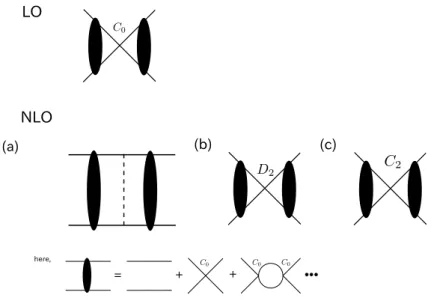
here + + +

...

Figure 3.2: The LO amplitude in the pionless theory. Solid lines are nucleon propagator. In this section, we consider pionless diagrams. A black bulb is the sum of all bubble diagrams.

I_n =−i µ

2

_4−DZ d^Dq

(2π)^Dq²ⁿ i

E−q⁰− _2M^q² +i

i

E+q⁰− _2M^q² +i

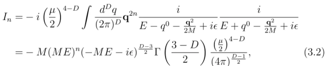
=−M(M E)ⁿ(−M E−i)^D²⁻³Γ

3−D 2

µ 2

4−D

(4π)^D⁻²¹, (3.2) whereDis the spacetime dimension which is eventually set to 4, andE is the total energy of the system. The parameterµof mass dimension is introduced to make the dimension ofI_n n+ 2 irrespective toD. I_ndoes not have a pole at D = 4, but it has a pole at D= 3, corresponding to the power(linear in the case of n = 0) divergence of the original integral at D = 4. It is the power divergence subtraction (PDS) regularization to subtract the poles at D= 3 as well as poles at D= 4. The counter term is

δI_n =−M(M E)ⁿµ

4π(D−3), (3.3)

and subtracted integral I_n^{P DS} is defined as I_n^{P DS} = lim

D→4(In+δIn) =−(M E)ⁿ M

4π

(µ+ip). (3.4) To obtain scattering amplitude at LO, one needs to sum all bubble diagrams in Fig.3.2:

iALO = −iC₀

1 + ^{M C}_4π⁰(µ+ip). (3.5)

(16)

One can get renormalization group equations by requiring that the physical scattering amplitude is independent of µ:

µ ∂

∂µiALO = 0. (3.6)

It is only possible when the coupling constant C₀ depends on µaccording to the following renormalization group equation:

µ ∂

∂µC₀ = M µ

4π C₀². (3.7)

Solving this equation, we obtain

C₀(µ) = 4π M

1

−µ+¹_a. (3.8)

When a is natural size(∼Λ), naive dimensional counting can be adopted to know the magnitude of coupling constants. In this case, it is convenient to take µ= 0.

In case of a ≤ 1 and µ → 0, the coupling constants are very large;

C_2n ∼ (4πaⁿ⁺¹)/(MΛⁿ). This difficulty can be avoided to take µ nonzero value in which case the coefficients may not be large; C2n ∼4π/(MΛⁿµⁿ⁺¹).

(17)

Chapter 4 Nuclear Effective Field Theory

In this chapter we will show brief review about nuclear effective field theory(NEFT) and phase shift analysis based on the EFT shown in the litera- ture. NEFT is low energy effective theory of nucleons based on symmetries of QCD and the freedoms of this theory is nucleons and pions.

4.1 Formalism

In this thesis, we will follow the notation in [14, 16, 17].

The Lagrangian for a nucleon system including pions is L =f_π²

8 Tr ∂^µΣ∂_µΣ^†

+f_π²ω

8 Tr m_qΣ +m_qΣ^† +N^†

i ~D₀+ D² 2M

N + ig_A

2 N^†σ_i ξ∂_iξ^†−ξ^†∂_iξ

−C₀^(s)O0^(s)+C₂^(s)

8 O^(s)2 −D₂^(s)ωTr(m^ξ)O0^(s)

− C₄^(s)

64 O₄^(s)+ E₄^(s)

8 ωTr(m^ξ)O^(s)₂ − D₄^(s) 2 ω²

Tr²(m^ξ) + 2Tr

(m^ξ)² O₀^(s)

−C₂^(SD)O2^(SD)+· · · . (4.1) Here g_A = 1.25 is the nucleon axial-vector coupling, and f_π = 131 MeV is

(18)

the pion-decay constant.

Σ =ξ² = exp

2iΠ f_π

, where, Π =

π⁰

√2 π⁺ π⁻ −^√^π⁰₂

!

, (4.2)

in which π^0,^± are pion fields. The chiral covariant derivative is Dµ = ∂µ+

1

2 ξ∂_iξ^†+ξ^†∂_iξ

andm^ξ = ¹₂ ξm_qξ^†+ξ^†m_qξ

andm_q = diag (m_u, m_d) is the quark mass matrix, ωTr(m^ξ) = m²_π = (137MeV)². The theory has a global (chiral) symmetry, SU(2)L×SU(2)R which is spontaneously broken to the vector subgroup SU(2)_V. Σ(x)→LΣ(x)R^†. The nucleon field transforms as

N(x)→U(x)N(x), (4.3)

where U(x) is defined as

ξ(x)→Lξ(x)U(x)^† =U(x)ξ(x)R^†. (4.4) Two nucleon operators for ¹S0 and ³S1 waves which appear in eq.(4.1) are defined as,

O^(s)0 =

N^TP_i^(s)N _†

N^TP_i^(s)N

, O^(s)2 =

N^TP_i^(s)N _†

N^TP_i^(s)∇²N

+h.c, O^(s)₄ =

N^TP_i^(s)N _†

N^TP_i^(s)∇⁴N

+h.c+2

N^TP_i^(s)∇²N _†

N^TP_i^(s)∇²N

, O^(s)4 =

N^TP_i⁽³^S¹⁾N _†

N^TP_i⁽³^D¹⁾N

+h.c. (4.5)

where P_i^(s) are the projection matrices with s specifying partial wave;

P_i⁽¹^S⁰⁾=(iσ2)(iτ2τi) 2√

2 ,

P_i⁽¹^S⁰⁾=(iσ₂σ_i)(iτ₂) 2√

2 . (4.6)

(19)

4.2 Amplitudes obtained by Fleming et al.

First of all, we show the result for the ¹S0 channel obtained by Fleming et.al [11]. In this paper, LO, NLO, and NNLO amplitudes are written A−1, A0, and A1 respectively:

A−1 = −4π M

1 γ+ip,

A0 = −A²₋1(ζ₁p²+ζ₂m²_π) (4.7)

+g_A² 2f²A²₋1

M m_π 4π

2

(γ²−p²) 4p² ln

1 + 4p² m²_π

− γ ptan⁻¹

2p m_π , A1 = A²0

A₋1

− A²₋1

ζ₃m²_π +ζ₄p²+ζ₅ p⁴ m²_π

+A0

M g_A² 8πf²

m²_π p

γ 2p ln

1 + 4p² m²_π

−tan⁻¹ 2p

m_π

+MA²₋1

4π

M g²_A 8πf²

2m⁴_π 4p³

(

2(γ²−p²) Im Li₂

−m_π m_π−2ip

−4γ pRe Li₂

−m_π m_π −2ip

−γ p π²

3 −(γ²+p²)

Im Li₂

m_π + 2ip

−m_π + 2ip

+γ 4pln²

1 + 4p² m²_π

−tan⁻¹ 2p

mπ

ln

1 + 4p² m²_π

) .

(20)

where, γ = 4π

M C0

+µ , ζ₁ = C₂

(C0)²

, ζ2 =

D₂

(C₀)² − g_A² 4f²

M 4π

2

ln µ²

m²_π

+ 1 m²_π

"

C₀⁽⁰⁾

(C₀)² + g²_A 2f²

M 4π

2

(γ²−µ²)

# ,

ζ₃ = −g²_A 2f²

M m_π 4π

C₂ (C₀)²

+ 1

m²_π

"

C₀⁽¹⁾

(C₀)² − (C₀⁽⁰⁾)² (C₀)³ −

g²_A 2f²

2 M 4π

3

(µ³−γ³)

#

−2γ m²_π

M g_A² 8πf²

"

C₀⁽⁰⁾

(C₀)² + g_A² 2f²

M 4π

2

(−µ²+γ²)

#

−2M γ 4π

M g_A² 8πf²

2

ln 2− 3 2

+m²_π D₄

(C₀)²− D²₂ (C₀)³

+

"

D₂⁽⁻¹⁾

(C₀)² −2D₂C₀⁽⁰⁾ (C₀)³ − g_A²

f² M γ

4π D₂ (C₀)²

#

+ζ₃^rad, ζ₄ =

"

C₂⁽⁻¹⁾

(C₀)² − 2C2C₀⁽⁰⁾ (C₀)³ − g_A²

f² M γ

4π C2

(C₀)²

# +m²_π

E4

(C₀)² − 2C2D2

(C₀)³

, (4.8) ζ₅ = m²_π

C₄

(C₀)² −(C₂)² (C₀)³

.

The parameters ζ₁ ∼ ζ₅ are dimensionless constants. Because of renormalization equation, quantities in square and curly brackets are separately µ independent.

To fit the phase shift to partial wave analysis data, they used the so-called good fit conditions. For the leading order operator C₀, it is

−1 a +r₀

2(p^∗)²−ip^∗ = 0. (4.9) This decide determines γ =−7.88MeV. For NLO, the condition is

ζ2 = γ²

m²_π ζ1− M 4π

g_A²M 8πf² log

1 + 2γ m_π

, (4.10)

At NNLO, ζ5 = 0 and the ranges p = 7 ∼ 80 MeV and p = 7 ∼ 200MeV were used for the fitting at NLO and NNLO respectively, with low momentum weighted more heavily.

NLO : ζ1 = 0.216; ζ2 = 0.0318;

NNLO : ζ₁ = 0.0777; ζ₂ = 0.0313; ζ₃ = 0.1831; ζ₄ = 0.245.

(21)

Note that the value of ζ₁ changes significantly from NLO to NNLO.

p(MeV)

1S₀

a)

δ(deg)

0 25 50 75

0 100 200 300 400

p(MeV)

1S₀

b)

δ(deg)

-50 0 50

0 100 200 300 400

Figure 4.1: Fit to the ¹S0 phase shift δ from Ref. [11]. The solid line is the Nijmegen fit [18] to the data. In a), the long dashed, short dashed, and dotted lines are the LO, NLO, and NNLO results respectively. In b) we show two other NNLO fits with a different choice of parameters.

The solid line is the Nijmegen phase shift analysis in each graph. The coupling constants given above are in Fig.4.1(a). At the LO fit, the error is about 48%, at the NLO, the error is 17%, and at the NNLO, the error is less than 1%. The KSW expansion gives improvement at this channel. In Fig4.1(b), the phase shift is fitted in constraints that the value of ζ₁ is close to its NLO value and ζ₄ ≤ζ₁.

Let us move on the ³S₁ channel. In this channel, there is a mixing with the ³D₁ channel.

The phase shift is expanded perturbatively.

δ¯₀ = ¯δ₀⁽⁰⁾+ ¯δ₀⁽¹⁾+ ¯δ₀⁽²⁾+· · · . (4.12) The phase shift at each order is given by

δ¯⁽⁰⁾₀ = 1 2iln

1 + ipM 2π A^SS₋1

, ¯δ₀⁽¹⁾ = pM 4π

A^SS0

1 + ^ipM_2π A^SS₋1

, δ¯⁽²⁾₀ = pM

4π

A^SS1

1 + ^ipM_2π A^SS₋1

−i pM

4π 2



 A^SS0

1 + ^ipM_2π A^SS₋1

!2

+ (A^SD0 )² 1 + ^ipM_2π A^SS₋1



. (4.13)

(22)

where the S-D mixing amplitude becomes , A^SD0 = √

2M g²_A 8πf²A^SS₋1

− 3m³_π 4p² +

m²_π

2p +3m⁴_π 8p³

tan⁻¹

2p m_π

+3γm²_π 4p² −γ

2

−γm²_π

4p² + 3γm⁴_π 16p⁴

ln

1 + 4p² m²_π

. (4.14)

(23)

A^SS₋1 =−4π M

1 γ +ip, A^SS0 =−h

A^SS₋1

i2

(ζ1p²+ζ2m²_π) +

hA^SS₋1

i2 g_A² 2f²

M m_π 4π

2

(γ²−p²) 4p² log

1 + 4p² m²_π

−γ ptan⁻¹

2p m_π , A^SS1 =[A^SS0 ]²

A^SS₋1

+ipM 4π

hA^SD0

i2

+A^SS0

M g²_A 8πf²

m²_π p

γ 2plog

1 + 4p² m²_π

−tan⁻¹ 2p

m_π

−h A^SS₋1

i2

ζ₃m²_π +ζ₄p²+ζ₅ p⁴ m²_π

+ hA^SS₋1

i2M 4π

M g_A² 8πf²

2"

−6γ²m³_π + 9γm⁴_π−3m⁵_π 4p²

+ log 2

9γm⁶_π

4p⁴ +3γm⁴_π

2p² −9m⁷_π

4p⁴ − 3m⁵_π p²

+

6p²+ 6m²_π− 3m⁴_π

4p² − 9m⁶_π 8p⁴

p²−γ² p tan⁻¹

p m_π

−γlog

1 + p² m²_π

−3m⁵_π

p³ +9m⁷_π 4p⁵

γtan⁻¹ p

m_π

− (γ² −p²) 4p log

1 + p²

m²_π +

9m⁷_π

8p⁵ + 3m⁵_π

2p³ − 9γm⁶_π

8p⁵ − 3γm⁴_π

4p³ +γm²_π p

×

γtan⁻¹ 2p

m_π

+ p 2log

1 + 4p² m²_π

+ 9m⁸_π

32p⁷ + 3m⁶_π

4p⁵ +3m⁴_π 4p³

(

2(γ²−p²)Im Li₂

−m_π m_π −2ip

−4γpRe Li₂

−mπ

m_π−2ip

− γpπ²

3 −(γ²+p²)

Im LI₂

mπ+2ip

−m_π+2ip

+ γ 4plog²

1 + 4p² m²_π

−tan⁻¹ 2p

m_π

log

1 + 4p² m²_π

)

+γ 9m⁸_π

32p⁶+3m⁶_π 4p⁴ + m⁴_π

2p²

tan⁻¹ 2p

m_π

− γ 2plog

1 + 4p² m²_π

² # . (4.15)

(24)

We have introduced the notations:

γ = 4π

M C₀ +µ, ζ1 = C₂

(C₀)²

, ζ₂ =

D₂

(C₀)² − g_A² 4f²

M 4π

2

log µ²

m²_π

+ 1 m²_π

"

C₀⁽⁰⁾

(C₀)² + g²_A 2f²

M 4π

2

(γ²−µ²)

# , ζ₃ =− g²_A

2f² M mπ

4π

C2

(C₀)²

− 1 m²_π

M 4π

M g_A² 8πf²

2

γ³−6m_πγ²− 7

2m²_πγ + 4m³_π

+ 1 m²_π

"

C₀⁽¹⁾

(C₀)² − (C₀⁽⁰⁾)² (C₀)³ − g_A²

f² M γ

4π C₀⁽⁰⁾ (C₀)² − M

4π

M g²_A 8πf²

2

4µγ²−6γµ²+ 4 3µ³

#

+m²_π D₄

(C₀)² −(D₂)² (C₀)³

+

"

D₂⁽⁻¹⁾

(C0)² − 2D₂C₀⁽⁰⁾ (C0)³ − g_A²

f² M γ

4π D₂

(C0)² −5M γ 4π

M g²_A 8πf²

2

ln µ²

m²_π

#

+ζ₃^rad, ζ₄ =

"

C₂⁽⁻¹⁾

(C0)² − 2C₂C₀⁽⁰⁾

(C0)³ −6M γ 4π

M g_A² 8πf²

2

ln µ²

m²_π

# +m²_π

E₄

(C0)² −2C₂D₂ (C0)³

,

−g²_A f²

M γ 4π

C₂ (C₀)²

− M 4π

M g_A² 8πf²

2

−3γ+ 6m_π), ζ₅ =m²_π

C₄

(C0)² − (C₂)² (C0)³

. (4.16)

By fitting to the data, they obtained the following values for these parameters,

NLO : ζ1 = 0.327; ζ2 =−0.0936; (4.17)

NNLO : ζ₁ = 0.432; ζ₂ =−0.0818; ζ₃ = 0.165; ζ₄ = 0.399.

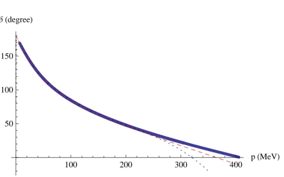
At LO, the phase shift has no free parameters. At NLO there is one free parameterξ₁, and the fit to the data is very good. However, at NNLO the fit of the phase shift to the data becomes worse at the momentum region more than p'50 MeV.

In the ³S₁ channel, the term expressed below appear in the scattering

(25)

p(MeV)

3S₁ δ 0(deg)−

0 50 100 150

0 100 200 300

Figure 4.2: The ³S₁ phase shift for NN scattering from Ref [11]. The solid line is the Nijmegen multi-energy fit [18], the long dashed line is the LO effective field theory result, the short dashed line is the NLO result, and the dotted line is the NNLO result. The dash-dotted line shows the result of including the parameter ζ5 which is higher order in the power counting.

(26)

amplitude,

A^SS1 '6 [A^SS₋1]² M 4π

M g²_A 8πf²

2

p³tan⁻¹ p

m_π

. (4.18)

For the momentum region p m_π, this term grows linearly with p. This is the source of the failure of the KSW power counting at NNLO in the ³S₁ channel. It is considered that such a term comes from the singularity of the tensor force near the origin, r = 0 in the coordinate space.

(27)

Chapter 5 Wilsonian renormalization group analysis

In this chapter we review Wilsonian renormalization group analysis in the NEFT.

5.1 Scaling dimensions

Let us consider the interaction Lagrangian L= ΣG_iOi whereG_i is coupling constant and Oi is corresponding operator. It is useful to consider the RG equations written in terms of dimensionless coupling constants defined as,

G_i(Λ)≡ g_i(Λ)

Λ^dⁱ⁻^D, (5.1)

where Λ is the floating cutoff,D is the dimension of spacetime, and d_i is the canonical dimension of the operatorOi. The RG equation of coupling g_i may be written as

dg_i

dt =βi(g), t ≡log Λ₀

Λ

. (5.2)

We are interested in the behavior of the coupling constants near the fixed point, so we substituteg_i =g^∗_i +δg_i to the RG equation, whereg_i^∗ is value of the coupling constant on the fixed point,β(g^∗) = 0, andδgi is small deviation from fixed point,

d

dtδg_i = ∂β_i

∂g_j

∗

g

≡A_ij(g^∗)δg_j. (5.3)

(28)

By diagonalizing A_ij, we get

du_i

dt =ν_iu_i, (5.4)

where ν_i⁰s are the eigenvalues and u⁰_is are the corresponding eigenvectors.

This RG equation may be integrated as, u_i(Λ) =u_i(Λ₀)

Λ Λ₀

₋νi

. (5.5)

The coupling are called irrelevant, marginal, and relevant whenν_i <0,ν_i = 0, and ν_i >0 respectively.

Suppose that coupling constant g_i(Λ) is written as g_i(Λ)∼g_i^∗+ Σ_kc_ik

Λ Λ₀

₋νk

, (5.6)

so dimensionful coupling constant becomes G_i(Λ)∼ g_i^∗

Λ^dⁱ⁻^D + Σ_kc_ik Λ^ν₀^k

Λ^dⁱ⁻^D+ν^k. (5.7) Counting powers of Λ₀ is the correct power counting.

5.2 Renormalization group equations

The Wilsonian RGEs for NEFT including pions are obtained in [19]

(29)

dx

dt = −x−

"

x²+ 2xy+y²+ 2xz+ 2yz +z²

#

−2(x+y+z)γ−γ², (5.8)

dy

dt = −3y−

"

1

2x² + 2xy+ 3

2y²+yz− 1 2z²

#

−(x+ 2y)γ− 1

2γ², (5.9)

dz

dt = −3z+

"

1

2x²+xy+1

2y²−xz−yz− 3 2z²

#

+(x+y−z)γ+1

2γ², (5.10)

du

dt = −3u−2(x+y+z)(u−γ)−2uγ+ 2γ², (5.11) and for γ,

dγ

dt =−γ. (5.12)

Here, we have introduced of dimensionless coupling constants, x≡ MΛ

2π²C₀^(S), y≡ MΛ³

2π² 4C₂^(S), z ≡ Λ³

2π²B^(S), u≡ MΛ³

2π² D^(S)₂ , u⁰ ≡ MΛ³ 2π² D₂^(T⁾. (5.13)

The nontrivial fixed point of the above RGEs relevant to the real two-nucleon system is found to be,

(x^?, y^?, z^?, u^?, γ^?) =

−1,−1 2,1

2,0,0

, (5.14)

which is identified with that found in the pionless NEFT given in Ref. [20].

(30)

The eigenvalues and corresponding eigenvectors are,

ν₁ = +1 : u₁ =





 1 1

−1 0 0





, ν₂ =−1 : u₂ =





 0

−1 1 0 0





,

ν₃ = −2 : u₃ =





 2

−1

−2 0 0





, ν₄ =−1 : u₄ =





 0 0 0 1 0





.

(5.15) This is only one operator with positive eigenvalue which corresponds to a relevant operator explained in the previous section. All the other operators are irrelevant. This aspect is very similar to KSW power counting in which only the contact interaction without derivatives is a relevant operator, and other operators are irrelevant, but pion contributions are different. In the KSW power counting, pion contributions are perturbative but the Wilsonian RGEs analysis implies that short-distance contributions of pions are included into contact interactions. Furthermore one of the contact interaction is relevant, so a part of short-distance pion contributions have to be treated as relevant.

The long-distance contributions of pions are irrelevant so one can treat them as perturbations.

(31)

Chapter 6 Computation of phase shifts of nucleon-nucleon scattering

In this chapter, we show the computation of nucleon-nucleon scattering phase shifts in NEFT based on the power counting found in [19].

6.1 Hybrid regularization

From the Wilsonian RG analysis described in the previous chapter, we think that it is necessary to make a decomposition of pion exchange contributions into its short-distance part and long-distance part. We first notice that the pion exchange can be written as

k²

k²+m²_π →1− m²_π

k²+m²_π. (6.1)

The first term may be viewed as the short-distance part, while the second term, which has a milder short-distance behavior, may be viewed as the long- distance part. It however still has a large contribution for short-distance, we therefore introduce a Gaussian damping factor,e⁻^k²^/λ², which suppresses the short-distance contributions,

− m²_π

k²+m²_π → − m²_π k²+m²_πe⁻^k

2

λ2, (6.2)

where λ is the cutoff scale, which is an analog of the floating cutoff in the Wilsonian RG analysis. All diagrams including pions are calculated with this damping factor.