X-ray Probing of the Matter Surrounding Accretion-Powered X-ray Pulsars

Surrounding Accretion-Powered X-ray Pulsars

Yuki Yoshida

Department of Physics, Graduate School of Science, Rikkyo University, 3-34-1 Nishi-Ikebukuro, Toshima, Tokyo 171-8501, Japan

A doctoral thesis submitted to the Department of Physics, Graduate School of Science, Rikkyo University

September 2018

ABSTRACT

Accretion-powered X-ray pulsar consists of a magnetized neutron star and a normal stellar companion. The magnetized neutron stars are astrophysical laboratories for testing theories of dense matter physics and propagation of radiation in strong magnetic fields. They are also good laboratories for study of an accretion flow onto a compact star, and for investigation of interactions between matters and X-rays. The X-ray emission lines, observed in their energy spectrum, provide information on the accretion flow and the interaction between intense X-rays and the accreting matter onto the neutron star in their strong magnetic field. The photoelectric absorption by the matter along the line of sight is also helpful to investigate the matter around the accretion-powered X-ray pulsars. We diagnostic the physical characteristic, such as the size, geometry, density and ionization state of the matter surrounding the accretion-powered X-ray pulsar through the X-ray spectroscopy, focusing on emission line as well as the photoelectric absorption edge.

In this thesis, we present the results of the Suzaku observation of 23 accretion-powered X-ray pulsars. From phase-averaged spectroscopies, iron K

emission lines were detected at almost 6.40 keV from the all the sources in our samples. Their emission mechanism is considered to be the fluorescent reprocessing of the X-rays from the X-ray pulsar by cold matter surrounding the X-ray sources. Detailed phase-resolved spectral analyses reveal clear flux modulations of the iron K

line with their rotation period of the neutron star, in the four sources; 4U 1907+097, 4U 1538-522, GX 301-2, and GX 1+4. We point out an apparent flux modulation of emission line with rotation period of neutron star due to the finite speed of light (we call this effect the “finite light speed effect”), if the mechanism of the line emission is a kind of reprocessing, such as the fluorescence by X-ray irradiation from X-ray pulsars.

This effect is applied to the observed pulse phase modulation of the iron line flux of GX 1+4.

We first discovered the significant modulation of the iron absorption K-edge depth with

pulse period from four pulsars; GX 301-2, Vela X-1, GX 1+4, and OAO 1657-415. The mod-

ulation of the iron K-edge depth can be reasonably explained by the following scenario. The

accreting matter along the magnetic filed line, which is constrained into a part of the Alfv´ en

shell, is responsible for the absorption edge. The constrained accreting matter co-rotates

with the neutron star spin because they are confined by the strong magnetic field of the pul-

sar. We further discuss the matter surrounding the accretion-powered X-ray pulsar based

on the knowledge provided by our analyses of the emission lines and absorption edge of iron.

1 Introduction 1

2 Review 3

2.1 X-ray Binary Source and Accretion . . . . 4

2.1.1 X-ray Binaries . . . . 4

2.1.2 Accretion in Binary System . . . . 5

2.2 Accretion-Powered X-ray Pulsars . . . . 10

2.2.1 General Picture . . . . 10

2.2.2 Accretion in X-ray Pulsars . . . . 10

2.2.3 X-ray Spectra . . . . 13

2.2.4 Emission Line . . . . 17

2.2.5 Classification of X-ray Pulsars . . . . 20

3 Instrument 25 3.1 Overview of Suzaku Satellite . . . . 26

3.2 X-ray Telescope . . . . 28

3.2.1 Performance and Calibration . . . . 28

3.3 X-ray Imaging Spectrometer . . . . 33

3.3.1 Overview . . . . 33

3.3.2 Performance and Calibration . . . . 35

3.3.3 Systematic Observational Effects and their Mitigation . . . . 38

3.3.4 Operation . . . . 40

3.4 Hard X-ray Detector . . . . 41

3.4.1 Overview . . . . 41

3.4.2 Performance and Calibration . . . . 43

3.5 Summary of the Mission . . . . 48

4 Observations 49 4.1 Data Reduction . . . . 50

4.2 Light Curves . . . . 51

4.2.1 BeXB Pulsars . . . . 51

4.2.2 SGXB Pulsars . . . . 57

4.2.3 LMXB Pulsars . . . . 63

4.3 Summary of Selected Sources . . . . 66

v

5 Data Analysis and Results 69

5.1 Phase-averaged Analysis . . . . 70

5.1.1 Phase-averaged Spectra . . . . 70

5.1.2 Modeling of Broadband Spectra . . . . 71

5.2 Phase-resolved Analysis . . . . 99

5.2.1 Selection of Sources . . . . 99

5.2.2 Pulse Period Determination . . . . 99

5.2.3 Spectral Fitting . . . 105

5.2.4 Investigating Statistical Significance of Variations . . . 112

5.3 Phase-resolved Analysis with High Intensity State Data . . . 118

5.3.1 Pulse Profiles . . . 118

5.3.2 Spectral Parameter Variations with Pulse Phase . . . 118

6 Discussion 123 6.1 Summary of the Results . . . 124

6.2 Nature of Iron Lines . . . 125

6.2.1 Fluorescent Iron K-line Emission and its Emission Region . . . 125

6.2.2 Finite Light Speed Effect . . . 128

6.3 Possible Origins of Modulating Absorption Edge Depth . . . 135

6.3.1 Two Spectral Components Influenced by Different Degree Absorption 137 6.3.2 Physical State Variation of Absorption Matter . . . 142

6.3.3 Geometric Variation of Absorption Matter . . . 146

6.4 Distribution of Iron Surrounding X-ray Pulsar . . . 151

6.4.1 Unified Picture . . . 151

6.4.2 Accreting Matter within Alfv´ en radius . . . 153

7 Conclusion 157

2.1 A schematic view of an X-ray binary . . . . 4

2.2 Classification of X-ray binaries . . . . 5

2.3 Roche lobe and equipotential surface of a binary system . . . . 7

2.4 Emission beam patterns from the poles of the NS . . . . 12

2.5 Energy of iron emission line and absorption K-edge . . . . 18

2.6 Corbet Diagram . . . . 22

3.1 Schematic view of the spacecraft . . . . 26

3.2 Picture of the XRT . . . . 28

3.3 Schematic view of Wolter-I type mirrors . . . . 28

3.4 Total effective area of the XRT . . . . 29

3.5 Off-axis angle dependence of the XRT . . . . 30

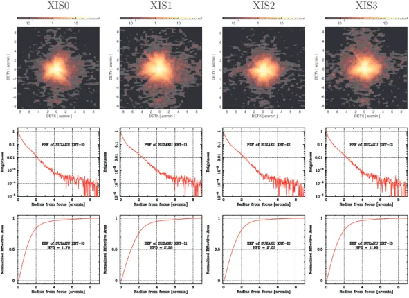
3.6 Typical X-ray image, PSF, and EEF of the XRT . . . . 31

3.7 Focus and optical axis of the XRT . . . . 32

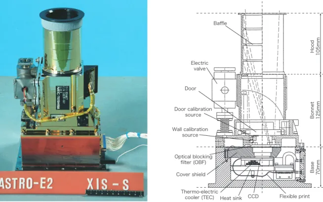
3.8 Picture and cross section of the XIS . . . . 33

3.9 Schematic view of a CCD chip in the XIS . . . . 34

3.10 Quantum efficiency of the XIS . . . . 35

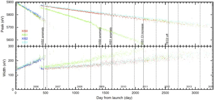
3.11 Energy resolution trend of the XIS . . . . 36

3.12 Typical NXB spectra of the XIS . . . . 37

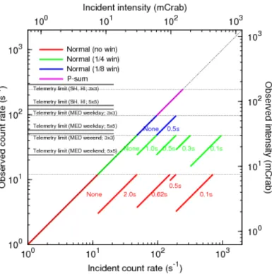
3.13 Incident versus observed count rates of a point-like source for the XIS detector 39 3.14 Picutre and cross section of the HXD . . . . 41

3.15 Array configuration of the HXD . . . . 42

3.16 Schematic view of the HXD . . . . 42

3.17 Total effective areas of the HXD . . . . 43

3.18 Angular response of the HXD . . . . 44

3.19 Typical NXB spectra of the HXD . . . . 45

3.20 In-orbit background of HXD . . . . 46

3.21 Short-term NXB variability of the HXD . . . . 47

4.1 Long-term light curves of Be X-ray pulsars . . . . 52

4.2 XIS and HXD-PIN light curves of A 0535+262 (ObsID=404055010) . . . . . 53

4.3 XIS and HXD-PIN light curves of GX 304-1 (ObsID=406060010) . . . . 53

4.4 XIS and HXD-PIN light curves of GX 304-1 (ObsID=905002010) . . . . 54

4.5 XIS and HXD-PIN light curves of GRO J1008-57 (ObsID=902003010) . . . . 54

vii

4.6 XIS and HXD-PIN light curves of GRO J1008-57 (ObsID=408044010) . . . . 54

4.7 XIS and HXD-PIN light curves of GRO J1008-57 (ObsID=907006010) . . . . 54

4.8 XIS and HXD-PIN light curves of EXO 2030+375 (ObsID=402068010) . . . 55

4.9 XIS and HXD-PIN light curves of EXO 2030+375 (ObsID=407089010) . . . 55

4.10 XIS and HXD-PIN light curves of 1A 1118-61 (ObsID=403049010) . . . . 55

4.11 XIS and HXD-PIN light curves of Cep X-4 (ObsID=409037010) . . . . 55

4.12 XIS and HXD-PIN light curves of Cep X-4 (ObsID=909001010) . . . . 56

4.13 XIS and HXD-PIN light curves of A 0535+262 (ObsID=100021010) . . . . . 56

4.14 XIS and HXD-PIN light curves of A 0535+262 (ObsID=404054010) . . . . . 56

4.15 XIS and HXD-PIN light curves of 1A 1118-61 (ObsID=403050010) . . . . 56

4.16 Long-term light curves of GX 301-2 . . . . 58

4.17 Long-term light curves of LMC X-4 and SMC X-1 . . . . 59

4.18 XIS and HXD-PIN light curves of OAO 1657-415 (ObsID=406011010) . . . . 60

4.19 XIS and HXD-PIN light curves of 4U 1909+07 (ObsID=405073010) . . . . . 60

4.20 XIS and HXD-PIN light curves of 4U 1907+097 (ObsID=401057010) . . . . 60

4.21 XIS and HXD-PIN light curves of 4U 1907+097 (ObsID=402067010) . . . . 60

4.22 XIS and HXD-PIN light curves of 4U 1538-522 (ObsID=407068010) . . . . . 61

4.23 XIS and HXD-PIN light curves of 4U 0114+65 (ObsID=406017010) . . . . . 61

4.24 XIS and HXD-PIN light curves of 4U 2206+54 (ObsID=402069010) . . . . . 61

4.25 XIS and HXD-PIN light curves of IGR J16393-4643 (ObsID=404056010) . . 61

4.26 XIS and HXD-PIN light curves of GX 301-2 (ObsID=403044010) . . . . 61

4.27 XIS and HXD-PIN light curves of GX 301-2 (ObsID=403044020) . . . . 61

4.28 XIS and HXD-PIN light curves of Vela X-1 (ObsID=403045010) . . . . 62

4.29 XIS and HXD-PIN light curves of Cen X-3 (ObsID=403046010) . . . . 62

4.30 XIS and HXD-PIN light curves of LMC X-4 (ObsID=702036020) . . . . 62

4.31 XIS and HXD-PIN light curves of SMC X-1 (ObsID=706030010) . . . . 62

4.32 Long-term light curves of Her X-1 . . . . 64

4.33 XIS and HXD-PIN light curves of Her X-1 (ObsID=101001010) . . . . 65

4.34 XIS and HXD-PIN light curves of 4U 1822-37 (ObsID=401051010) . . . . 65

4.35 XIS and HXD-PIN light curves of 4U 1626-67 (ObsID=400015010) . . . . 65

4.36 XIS and HXD-PIN light curves of 4U 1626-67 (ObsID=405044010) . . . . 65

4.37 XIS and HXD-PIN light curves of GX 1+4 (ObsID=405077010) . . . . 66

4.38 XIS and HXD-PIN light curves of 4U 1954+31 (ObsID=907005010) . . . . . 66

5.1 Phase-averaged, background-subtracted XISs and HXD spectra of A 0535+262 (ObsID=100021010) . . . . 74

5.2 Phase-averaged, background-subtracted XISs and HXD spectra of A 0535+262 (ObsID=404054010) . . . . 74

5.3 Phase-averaged, background-subtracted XISs and HXD spectra of A 0535+262 (ObsID=404055010) . . . . 75

5.4 Phase-averaged, background-subtracted XISs and HXD spectra of GX 304-1 (ObsID=406060010) . . . . 75

5.5 Phase-averaged, background-subtracted XISs and HXD spectra of GX 304-1

(ObsID=905002010) . . . . 76

5.6 Phase-averaged, background-subtracted XISs and HXD spectra of GRO J1008- 57 (ObsID=902003010) . . . . 76 5.7 Phase-averaged, background-subtracted XISs and HXD spectra of GRO J1008-

57 (ObsID=907006010) . . . . 77 5.8 Phase-averaged, background-subtracted XISs and HXD spectra of GRO J1008-

57 (ObsID=408044010) . . . . 77 5.9 Phase-averaged, background-subtracted XISs and HXD spectra of EXO 2030+375

(ObsID=402068010) . . . . 78 5.10 Phase-averaged, background-subtracted XISs and HXD spectra of EXO 2030+375

(ObsID=407089010) . . . . 78 5.11 Phase-averaged, background-subtracted XISs and HXD spectra of 1A 1118-61

(ObsID=403049010) . . . . 79 5.12 Phase-averaged, background-subtracted XISs and HXD spectra of 1A 1118-61

(ObsID=403050010) . . . . 79 5.13 Phase-averaged, background-subtracted XISs and HXD spectra of Cep X-4

(ObsID=409037010) . . . . 80 5.14 Phase-averaged, background-subtracted XISs and HXD spectra of Cep X-4

(ObsID=909001010) . . . . 80 5.15 Phase-averaged, background-subtracted XISs and HXD spectra of OAO 1657-

415 (ObsID=406011010) . . . . 81 5.16 Phase-averaged, background-subtracted XISs and HXD spectra of 4U 1909+07

(ObsID=405073010) . . . . 81 5.17 Phase-averaged, background-subtracted XISs and HXD spectra of 4U 1907+097

(ObsID=401057010) . . . . 82 5.18 Phase-averaged, background-subtracted XISs and HXD spectra of 4U 1907+097

(ObsID=402067010) . . . . 82 5.19 Phase-averaged, background-subtracted XISs and HXD spectra of 4U 1538-

522 (ObsID=407068010) . . . . 83 5.20 Phase-averaged, background-subtracted XISs and HXD spectra of 4U 0114+65

(ObsID=406017010) . . . . 83 5.21 Phase-averaged, background-subtracted XISs and HXD spectra of 4U 2206+54

(ObsID=402069010) . . . . 84 5.22 Phase-averaged, background-subtracted XISs and HXD spectra of IGR J16393-

4643 (ObsID=404056010) . . . . 84 5.23 Phase-averaged, background-subtracted XISs and HXD spectra of GX 301-2

(ObsID=403044010) . . . . 85 5.24 Phase-averaged, background-subtracted XISs and HXD spectra of GX 301-2

(ObsID=403044020) . . . . 85 5.25 Phase-averaged, background-subtracted XISs and HXD spectra of Vela X-1

(ObsID=403045010) . . . . 86 5.26 Phase-averaged, background-subtracted XISs and HXD spectra of Cen X-3

(ObsID=403046010) . . . . 86 5.27 Phase-averaged, background-subtracted XISs and HXD spectra of LMC X-4

(ObsID=702036020) . . . . 87

5.28 Phase-averaged, background-subtracted XISs and HXD spectra of SMC X-1 (ObsID=706030010) . . . . 87 5.29 Phase-averaged, background-subtracted XISs and HXD spectra of Her X-1

(ObsID=101001010) . . . . 88 5.30 Phase-averaged, background-subtracted XISs and HXD spectra of 4U 1822-37

(ObsID=401051010) . . . . 88 5.31 Phase-averaged, background-subtracted XISs and HXD spectra of 4U 1626-67

(ObsID=400015010) . . . . 89 5.32 Phase-averaged, background-subtracted XISs and HXD spectra of 4U 1626-67

(ObsID=405044010) . . . . 89 5.33 Phase-averaged, background-subtracted XISs and HXD spectra of GX 1+4

(ObsID=405077010) . . . . 90 5.34 Phase-averaged, background-subtracted XISs and HXD spectra of 4U 1954+31

(ObsID=907005010) . . . . 90 5.35 X-ray folded spectrum of A 0535+262 (ObsID=100021010) with best-fit model 92 5.36 X-ray folded spectrum of A 0535+262 (ObsID=404054010) with best-fit model 92 5.37 X-ray folded spectrum of A 0535+262 (ObsID=404055010) with best-fit model 92 5.38 X-ray folded spectrum of GX 304-1 (ObsID=406060010) with best-fit model . 92 5.39 X-ray folded spectrum of GX 304-1 (ObsID=905002010) with best-fit model . 93 5.40 X-ray folded spectrum of GRO J1008-57 (ObsID=902003010) with best-fit

model . . . . 93 5.41 X-ray folded spectrum of GRO J1008-57 (ObsID=907006010) with best-fit

model . . . . 93 5.42 X-ray folded spectrum of GRO J1008-57 (ObsID=408044010) with best-fit

model . . . . 93 5.43 X-ray folded spectrum of EXO 2030+375 (ObsID=402068010) with best-fit

model . . . . 93 5.44 X-ray folded spectrum of EXO 2030+375 (ObsID=407089010) with best-fit

model . . . . 93 5.45 X-ray folded spectrum of 1A 1118-61 (ObsID=403049010) with best-fit model 94 5.46 X-ray folded spectrum of 1A 1118-61 (ObsID=403050010) with best-fit model 94 5.47 X-ray folded spectrum of Cep X-4 (ObsID=409037010) with best-fit model . 94 5.48 X-ray folded spectrum of Cep X-4 (ObsID=909001010) with best-fit model . 94 5.49 X-ray folded spectrum of OAO 1657-415 (ObsID=406011010) with best-fit model 94 5.50 X-ray folded spectrum of 4U 1909+07 (ObsID=405073010) with best-fit model 94 5.51 X-ray folded spectrum of 4U 1907+097 (ObsID=401057010) with best-fit model 95 5.52 X-ray folded spectrum of 4U 1907+097 (ObsID=402067010) with best-fit model 95 5.53 X-ray folded spectrum of 4U 1538-522 (ObsID=407068010) with best-fit model 95 5.54 X-ray folded spectrum of 4U 0114+65 (ObsID=406017010) with best-fit model 95 5.55 X-ray folded spectrum of 4U 2206+54 (ObsID=402069010) with best-fit model 95 5.56 X-ray folded spectrum of IGR J16393-4643 (ObsID=404056010) with best-fit

model . . . . 95

5.57 X-ray folded spectrum of GX 301-2 (ObsID=403044010) with best-fit model . 96

5.58 X-ray folded spectrum of GX 301-2 (ObsID=403044020) with best-fit model . 96

5.59 X-ray folded spectrum of Vela X-1 (ObsID=403045010) with best-fit model . 96 5.60 X-ray folded spectrum of Cen X-3 (ObsID=403046010) with best-fit model . 96 5.61 X-ray folded spectrum of LMC X-4 (ObsID=702036020) with best-fit model . 96 5.62 X-ray folded spectrum of SMC X-1 (ObsID=706030010) with best-fit model . 96 5.63 X-ray folded spectrum of Her X-1 (ObsID=101001010) with best-fit model . 97 5.64 X-ray folded spectrum of 4U 1822-37 (ObsID=401051010) with best-fit model 97 5.65 X-ray folded spectrum of 4U 1626-67 (ObsID=400015010) with best-fit model 97 5.66 X-ray folded spectrum of 4U 1626-67 (ObsID=405044010) with best-fit model 97 5.67 X-ray folded spectrum of GX 1+4 (ObsID=405077010) with best-fit model . 97 5.68 X-ray folded spectrum of 4U 1954+31 (ObsID=907005010) with best-fit model 97 5.69 Energy-divided pulse profile of OAO 1657-415 during whole observation . . . 101 5.70 Energy-divided pulse profile of 4U 1909+07 during whole observation . . . . 101 5.71 Energy-divided pulse profile of 4U 1907+097 (ObsID=401057010) during whole

observation . . . 102 5.72 Energy-divided pulse profile of 4U 1907+097 (ObsID=402067010) in whole

observation . . . 102 5.73 Energy-divided pulse profile of 4U 1538-522 during whole observation . . . . 103 5.74 Energy-divided pulse profile of GX 301-2 (ObsID=403044020) during whole

observation . . . 103 5.75 Energy-divided pulse profile of Vela X-1 in whole observation . . . 104 5.76 Energy-divided pulse profile of GX 1+4 in whole observation . . . 104 5.77 Results of phase-sliced spectroscopy in Suzaku data of OAO 1657-415 during

whole observation . . . 107 5.78 Results of phase-sliced spectroscopy in Suzaku data of 4U 1907+097 (Ob-

sID=401057010) whole observation . . . 108 5.79 Results of phase-sliced spectroscopy in Suzaku data of 4U 1907+097 (Ob-

sID=402067010) whole observation . . . 109 5.80 Results of phase-sliced spectroscopy in Suzaku data of 4U 1909+07 whole ob-

servation . . . 109 5.81 Results of phase-sliced spectroscopy in Suzaku data of 4U 1538-522 whole ob-

servation . . . 110 5.82 Results of phase-sliced spectroscopy in Suzaku data of GX 301-2 (ObsID=403044020) whole observation . . . 110 5.83 Results of phase-sliced spectroscopy in Suzaku data of Vela X-1 whole obser-

vation . . . 111 5.84 Results of phase-sliced spectroscopy in Suzaku data of GX 1+4 whole observation111 5.85 Ratios of phase-resolved spectra normalized by a power-law model with pho-

ton index of 2.0 . . . 113 5.86 Phase-resolved spectra subtracted the best-fit continuum model of phase-

averaged broadband fitting . . . 114 5.87 Spectral ratio between two phase-resolved and results of the fitting of GX 301-

2 (ObsID=403044020) with data during whole observation . . . 116 5.88 Spectral ratio between two phase-resolved and results of the fitting of Vela X-1

with data during whole observation . . . 117

5.89 Spectral ratio between two phase-resolved and results of the fitting of GX 1+4 with data during whole observation . . . 117 5.90 Energy-divided pulse profile of OAO 1657-415 during the selected time interval 119 5.91 Results of phase-sliced spectroscopy in Suzaku data of OAO 1657-415 during

selected time interval . . . 119 5.92 Ratios of phase-resolved spectra normalized by a power-law model with pho-

ton index of 2.0 of OAO 1657-415 during the selected time interval . . . 121 5.93 Spectral ratio between two phase-resolved and results of the fitting of OAO 1657-

415 with data during selected time interval . . . 122 6.1 Diagram EW of iron K

line versus N

or, HR η . . . 125 6.2 A schematic picture of the assumed situation of homogenously distributed

matter . . . 127 6.3 Geometry used in the Monte Carlo simulation for the finite light speed effect 129 6.4 Examples of the simulated folded light curves of the fluorescent lines . . . 130 6.5 Relation between the amplitude of the flux modulation of the fluorescent lines

and the angle of β . . . 131 6.6 Distribution of calculated amplitude of the intensity modulation of the fluo-

rescent line on a two-dimensional map of i and β . . . 132 6.7 Flux modulation of the iron line and the pulse shape of GX 1+4 . . . 133 6.8 Phase-resolved spectral ratios to phase-averaged spectrum . . . 138 6.9 Example of the simulated spectra composed of direct and reflect X-ray com-

ponents . . . 140 6.10 Resultant edge depths as a function of the photon flux of the reflect component141 6.11 The simulated spectra assuming the X-ray reflection . . . 141 6.12 The ionization and recombination timescales . . . 143 6.13 Particle density plotted as function of the distance from the NS . . . 144 6.14 A schematic picture of the assumed situation of the absorbing matter co-

rotating with the NS spin . . . 146 6.15 Particle density plotted as function of the distance from the NS . . . 149 6.16 Resultant χ

values and sum of depths of the two absorption edge components

as a function of energy of the iron K-edge for GX 301-2 . . . 154 6.17 Resultant χ

values and sum of depths of the two absorption edge components

as a function of energy of the iron K-edge for Vela X-1 . . . 154 6.18 Resultant χ

values and sum of depths of the two absorption edge components

as a function of energy of the iron K-edge for GX 1+4 . . . 154 6.19 Resultant χ

values and sum of depths of the two absorption edge components

as a function of energy of the iron K-edge for OAO 1657-415 . . . 154

6.20 Particle density plotted as function of the distance from the NS . . . 155

3.1 Details of the Suzaku mission . . . . 48

4.1 Suzaku observation list of BeXB pulsars . . . . 53

4.2 Suzaku observation list of SGXB pulsars . . . . 57

4.3 Suzaku observation list of LMXB pulsars . . . . 63

4.4 Parameters of selected sources . . . . 67

5.1 List of applied spectral model components representing the phase-averaged spectra of APXPs . . . . 91

5.2 Best-fit spectral parameters obtained by fitting the phase-averaged spectra of APXPs . . . . 98

5.3 Revealed barycentric pulsation period of samples for phase-resolved spectral analysis . . . . 99

5.4 Results of χ

tests to investigate the modulation in the iron K

line flux and the depth of iron K-edge with pulse phase . . . 112

5.5 The amplitude of the iron line flux modulation with pulse phase . . . 115

5.6 Results of fitting spectral ratios around iron K-edge . . . 116

5.7 Results of χ

tests to investigate the modulation in the iron K

line flux and the depth of iron K-edge with pulse phase . . . 120

5.8 Results of fitting spectral ratios around iron K-edge . . . 121

6.1 Estimated column density of absorbing matter and X-ray luminosities . . . . 135

6.2 Estimated magnetic field strengths and Alfv´ en radii . . . 147

xiii

Introduction

Soon after the first X-ray observation with the satellite, rapid and sometimes periodic variations in the X-ray intensity of many point-like X-ray sources were discovered. With combination of observational results with optical and X-ray telescopes, it have been demon- strated that these X-ray sources are members of binary systems, namely X-ray binaries, which consist of a normal star and a collapsed star. In the system, matter streams from the normal star onto the nearby collapsed star with an intense gravitational field. Most of point X-ray sources discovered in our Galaxy belong to this class. The first discovered extra-solar X-ray source, Scorpius X-1 (Giacconi et al. 1962), was also identified as the X-ray binary system. Further studies suggested that the X-ray luminosity of Scorpius X-1 was about ten thousand times the total luminosity of the Sun, integrated over the all wavelength. In later the optical counterpart of Scorpius X-1 was identified to a faint 13th magnitude star, which puzzled astronomers to understand the cause of X-ray emission from the source. On the basis of these sparkling results, the concept of mass accretion on to a compact object was considered to explain the presence of strong X-ray emission from extra-solar sources, where gravitational potential energy of accreted matter is converted into kinetic energy, which are released in a form of X-rays when the matter decelerates through a radiative shock and settles onto the stellar surface.

An “accretion-powered X-ray pulsar (APXP)” is a subclass of the X-ray binaries, which consists of a rotating neutron star (NS) involving strong magnetic field, orbiting a normal star. The NS has its typically radius of 10 km and mass of 1.4M

(M

is the solar mass;

1.99 × 10

g) and then its core has higher density than nuclear matter (2.3 × 10

g cm

).

In the APXP, mass transfer from the companion star to the NS occurs and the matter from the stellar companion falls toward the NS, as forming a so-called accretion disk around the NS. Eventually the accretion matter is channeled by the strong magnetic field of the NS, and forms a columnar geometry. Although this general picture is widely accepted, how gas flows from the circumstellar accretion disk into the magnetosphere of the rapidly rotating NS and eventually to the NS surface is a complex and as yet unsolved problem.

Past observations have revealed that most of the APXPs exhibit prominent emission lines from neutral iron atoms at 6.4 keV as well as their absorption K-edge at 7.1 keV (e.g., White et al. 1983; Nagase 1989). These iron lines from the APXPs are considered to be

1

produced through fluorescence of nearby cold matters illuminated by X-rays with energies above the ionization energy from compact stars (Koyama 1985; Inoue 1985; Makino et al.

1985; Makishima 1986; Nagase 1989). Since the emission line and absorption K-edge of iron can be hence associated with each other, a detailed investigation of them is necessary for diagnostics of their mechanism and origin. Identification of emission lines (ionization state of elements) and observed changes in line parameters with time and source luminosity provide important information on the line emitting regions such as relatively thick inhomogeneous and clumpy stellar wind from the companion star (Sako et al. 2002; Watanabe et al. 2006), surface or photosphere of the companions star, and probably the accreting matter around the Alfv´ en shell (Pravdo et al. 1977; Basko 1980). The observed absorption edge parameter provides us with the information of the matter placed between the X-ray source and an observer. This information is an independent one from those obtained by the emission line.

Therefore, a thorough investigation of not only the emission lines but also the absorption edge in the spectrum of APXPs will provide new information on the matter surrounding the NS, e.g., the accreting matter onto the NS interacted with its strong magnetic field.

In this thesis, we analyzed the data of the Suzaku observation of the several APXPs. The main aim of this thesis is to reveal the distribution of the matter in APXP systems through the understanding of the physical mechanisms relevant to the production of emission lines, especially the 6.4 keV iron K

line emissions, as well as absorption K-edge of iron at 7.1 keV.

This thesis is organized as below. Chapter 2 gives an introduction to the close X-ray binary systems and the APXPs. In chapter 3 we show instrumentation of Suzaku. Chapter 4 shows the Suzaku observations of APXPs. In chapter 5 the Suzaku data of APXPs were analyzed.

In chapter 6, we make discussion with the results of our analysis and provide interpretations

of them. Chapter 7 is the conclusion of this thesis.

Review

Contents

2.1 X-ray Binary Source and Accretion . . . . 4

2.1.1 X-ray Binaries . . . . 4

2.1.2 Accretion in Binary System . . . . 5

2.2 Accretion-Powered X-ray Pulsars . . . . 10

2.2.1 General Picture . . . . 10

2.2.2 Accretion in X-ray Pulsars . . . . 10

2.2.3 X-ray Spectra . . . . 13

2.2.4 Emission Line . . . . 17

2.2.5 Classification of X-ray Pulsars . . . . 20

3

2.1 X-ray Binary Source and Accretion

2.1.1 X-ray Binaries

A binary system consists of two stars, which orbit around a common center of mass, that is they are gravitationally bound to each other. In very general terms, one can simply define X-ray binaries as systems that contain a compact object orbiting an optical companion, which is a sub-class of binary systems. They are close binary systems and there exists a mass-transfer from the companion star to the compact object. The falling or accreting matter toward the compact object often forms a so-called accretion disk around the compact object. Gravitational energy of the accreted matter heats the gas around the compact object to very high temperatures (10

to 10

K), and the gas brightly shines in X-ray regime (L

= 10

–10

ergs s

). Figure 2.1 shows a sketch of an X-ray binary system as it would be seen by a nearby observer (Klochkov 2007). There are several classification schemes depending on whether the emphasis is put on the type of the compact star or the physical properties of the optical star. Indicating by a tree-diagram depicting all the different subsystems in Figure 2.2, X-ray binaries divide up into black hole systems, NS binaries or cataclysmic variables (if the compact object is a white dwarf). The X-ray binaries are also conventionally classified as low mass X-ray binaries (LMXBs) and high mass X-ray binaries (HMXBs) according to the mass of the companion star. HMXBs contain early-type (O or B) companions (typically mass of M

> 10M

), while the spectral type of the optical star (in general M

< 1M

) in LMXBs is later than A. The classification of this companion star closely relate to the mode of mass-transfer mechanism and the environment surrounding the X-ray source.

Figure 2.1: A schematic view of an X-ray binary (Klochkov 2007).

XRB

Black Holes Neutron stars White dwarf

HMXB

HMXB LMXB LMXB

- (Classical) novae - Recurrent novae - Dwarf novae - Polars - VY Sculptoris - AM Canum - SW Sextantis

atoll

Z

BeXB SGXB

- disc-fed - wind-fed - SFXT - Transient - Persistent

Figure 2.2: Classification of X-ray binaries (Reig 2011).

2.1.2 Accretion in Binary System

One of the most efficient energy sources is known as an accretion onto a compact star, where the gravitational energy is efficiently converted to kinetic or thermal energy. The X-ray binaries are powered by this mechanism. If a particle falls onto a compact object with a mass M

and a radius R

from an infinite distance along a radial direction, the velocity at r from the center of the compact object is represented by a free fall velocity, given by

v

(r) =

√ 2GM

r , (2.1)

where G is the gravitational constant. Assuming that all the kinetic energy liberated is converted to radiation at the surface of the star, the total luminosity, L

, can be given by

L

= 1 2

M v ˙

(R

)

= GM

M ˙

R

, (2.2)

where ˙ M is the steady accretion rate (in mass per unit time). For a modest mass transfer rate of ˙ M ∼ 10

g s

, one expects a luminosity of 10

ergs s

. If it emits thermally from an area of a few times the size of the compact object, this radiation must predominantly fall in the X-ray band ( ∼ 1 keV). Higher characteristic temperatures occur when the NS has a strong magnetic field that funnels all accreting matter onto two small areas near its poles, or when for some reason the emission is (partially) non-thermal.

The liberated accreted energy L

is sometimes expressed in a unit of its Eddington

luminosity L

. Assuming spherical symmetry, fully ionized accreted matter consisting of

only hydrogen, and a steady accretion, L

represents the maximum possible luminosity,

above which a star starts blowing away its outer layers by radiation pressure. L

can be

derived by equating the gravitational force exerted by a star to the radiation force by fully

ionized hydrogen plasma, and is given by L

= 4πGM

m

c

σ

∼ 1.3 × 10

( M

M

)

ergs s

, (2.3)

where m

is the proton mass (m

= 1.7 × 10

g), and σ

is the Thomson scattering cross section (σ

= 6.7 × 10

cm

).

Mass transfer from the companion star to the compact star takes place by different mechanisms according to some physical properties of binary system. In the HMXBs, the matter from the companion star generally accretes through stellar wind or equatorial disk.

On the other hand, in the LMXBs, mass transfer occurs through the inner Lagrange point–

the point where sum of gravitational forces and centrifugal force equals to zero. In the following section, we provide description of the different aspects of accreting mechanisms.

2.1.2.1 Roche lobe overflow

A star with certain mass and radius consists of spherical equipotential surfaces around it. By the presence of second star, the equipotential surfaces of a star appear no longer symmetric. They distort from spherical geometry and represent by a combined effective potential of both the stars, known as the Roche potential. The Roche potential is given by

Φ

(r) = − GM

| r − r

| − GM

| r − r

| − 1

2 | ω × r |

, (2.4)

where M

and M

are the masses of two stars, r

and r

are the position vectors of its centers, and ω is the orbital angular velocity vector (Frank et al. 2002). The first and second terms are the gravitational potential, and the third one is the centrifugal potential.

Close to each star, the potential is dominated by the gravitational potential of the star making the equipotential plane almost spherical. Figure 2.3 shows sections in the orbital plane of equipotential surfaces of Φ

. The some extremum points are called the Lagrange points, where the net force on a test particle cancel out, and the number of them is five. It can be seen that the lobes of both the stars are connected at a point called first Lagrange point L

. This equipotential surface is called Roche lobe. By some reasons, one of the stars in the binary system may increase in radius, or the binary separation may shrink and then one star fills its own Roche lobe. Then the gravitational attraction force of the compact star can gradually remove material from the companion star and the mass transfer occurs via the Lagrange point L

(Frank et al. 2002; Longair 2011). Such type of mass transfer mechanism is known as “Roche-lobe overflow” and is applicable to systems where accretion disk are formed especially in LMXBs and in a few HMXBs.

If the matter in-falling on the compact object has sufficient specific angular momentum J , it will form a rotationally flattened disk around the compact object referred as the accretion disk. Assuming that the local circular velocity of the accreting matter can be approximated by Keplerian, the specific angular momentum J at the radius r is given by

J = Ω

r

= √

GM

r, (2.5)

where Ω

= √

GM

/r

is an angular velocity at the radius of r. This formula can be rewrote for a radius,

R

= J

GM

. (2.6)

Here R

is the circularization radius for the matter with specific angular moment J. If the accretion matter satisfies this condition, which means that the matter has an adequate angular momentum, the Keplerian accretion disk can be formed.

The estimation of circularization radius can also constrain the upper limit of the disk size.

In other words, this relates to a distance where the disk begins to form. For the accretion via the Roche lobe overflow in LMXB system, the circularization radius can be simply described as

R

∼ 3.5 × 10

( M

M

) ( P

1 hr

)

cm, (2.7)

where, P

is the orbital period of binary system and M

is the mass of companion star (Frank et al. 2002). As it can be clearly seen, the R

is sufficiently larger than the size of compact object for both NSs and white dwarfs (10

and 10

cm respectively). Therefore an accretion disk is always expected to form during the process of Roche-lobe overflow.

Figure 2.3: Sections in the orbital plane of the Roche equipotentials Φ

=constant, for a

binary system with mass ratio q = M

/M

= 0.25 (Frank et al. 2002). Shown are the centre

of mass and Lagrange points L

–L

. The equipotentials are labelled 1–7 in order of increasing

Φ

.

2.1.2.2 Capture from the Stellar Wind

Significant amount of the stellar mass of the companion may be ejected in the form of a stellar wind, during its life, and a fraction of this material be captured gravitationally by the compact object. Foregoing accretion mechanism is called “stellar wind accretion” and is usually applicable to the HMXBs (Bondi & Hoyle 1944; Davidson & Ostriker 1973). They are very luminous in nature and hence most of the first sources to be discovered like Vela X-1 fall in this category.

Mass loss rate from these early type companions are between 10

–10

M

yr

and are in the form of intense, supersonic stellar winds. This wind velocity greatly exceeds the sound velocity (c

) the local medium given by c

∼ 10 (

10⁴K

) km s

. The accreting gas as a result is not in the form of hydrostatic equilibrium. In general only a small fraction of the wind is accreted, in contrast to the Roche lobe overflow case where almost all the mass is captured by the accreting component. A compact object with mass M

and moving with relative velocity v

through a medium with sound speed c

will gravitationally capture matter along a roughly cylindrical region with its axis along the relative wind direction (Davidson &

Ostriker 1973; Lamb et al. 1973). The radius R

of the cylinder also called the accretion radius or gravitational capture radius is given by

R

= 2GM

v

+ c

, (2.8)

where v

= v

+v

, v

is an orbital velocity of the compact object, and v

is a stellar wind velocity (see Bondi & Hoyle 1944; Blondin et al. 1990). In most cases, c

≪ v

and the term of c

can be neglected. Since v

is of the order of 1000–2000 km s

and v

is considerably lower, R

is estimated as ∼ 10

cm. The mass accretion rate ˙ M is described with R

, v

, and density of the wind ρ

as

M ˙ = πR

ρ

v

. (2.9) Since the stellar winds are generally inhomogeneous, ρ

and ˙ M fluctuate largely. These therefore make the compact object with massive companion highly time variable in X-ray.

For the case of the stellar wind accretion, the specific angular momentum J is given by J = 1

4 Ω

(R

)

, (2.10)

where Ω

is the orbital angular velocity. Following Frank et al. (2002), the circularization radius for the stellar wind accretion can be derived to be

R

∼ 1.3 × 10

( M

M

)

( P

10 d

)

cm. (2.11)

For M

= 10M

, this is greater than the size of the compact object in case of NSs or white

dwarfs. So in case of the stellar wind accretion, accretion disks may be formed (Boerner

et al. 1987), but are small in size. Anyway, it is difficult to decide whether the disk formation

condition (Equation 2.6) is satisfied.

2.1.2.3 Mass accretion from the equatorial disk

Mass loss from the equatorial disk is the mechanism of mass transfer for HMXBs with B-emission companion stars (Be stars), which is a dwarf, sub-giant or giant O/Be star (luminosity class III–V; Reig 2011). So, Be/X-ray binary (BeXB) is a subclass of HMXBs.

In these binary systems, the Be companion star rapidly rotates, shows, at irregular time intervals, outbursts of equatorial mass ejection which produce a rotating ring of gas around the star, giving rise to hydrogen emission lines in the optical spectrum. These systems typically have a large orbital period, moderate eccentricity, and being a non-supergiant system, the Be star lies deep within the Roche lobe. The abrupt accretion of matter onto the NS occurs while passing through the circumstellar disk of the Be companion. The ejected matter from the equatorial disk is captured at a distance R

from the NS as in the case of wind-fed HMXBs and the same description can be assumed to the first approximation.

Strong X-ray outbursts triggered by such the abrupt mass accretion are often observed

from these system (Okazaki & Negueruela 2001). During such outbursts, the X-ray emission

can be transiently enhanced by a large factor. Most BeXBs are transient sources and display

two types of outbursts, such as (i) short, periodic (according to orbital period of binary

system), less luminous Type I outbursts ( ⩽ 10

–10

ergs s

), lasting for a few days,

occurring at the phase of the periastron passage; and (ii) giant, longer, Type II outbursts

(L

⩾ 10

ergs s

), lasting for several weeks to months, occurring when a large fraction of

matter is accreted from the disk of Be star no showing any clear orbital dependence. Type

II outbursts are sometimes followed by smaller recurrent Type I outbursts. It also shows a

persistent low luminosity X-ray emission during quiescence (Negueruela et al. 1998).

2.2 Accretion-Powered X-ray Pulsars

This thesis aims at studying the matter surrounding the highly magnetized NSs through emission lines and the absorption features found in their X-ray spectra. Following sections, we describe the properties of the X-ray binaries especially containing a strongly magnetized NS and a normal stellar companion as a mass donor, so called “accretion-powered pulsar”.

2.2.1 General Picture

The first discovered accretion-powered pulsar is Centaurus X-3 (Cen X-3) in 1971 (Giac- coni et al. 1971) with the Uhuru satellite. Cen X-3 exhibits a pulsed variation with a period of 4.84 s only in the X-ray flux. In the accretion-powered pulsar, since the NS has a strong magnetic field, typically 10

G, the accretion flow will be disrupted at some distance from the NS by the magnetic field, and channeled to the magnetic poles of the NS, where most of X-rays originate from the conversion of gravitational potential energy into kinetic or thermal energy with a shock wave heating as described in § 2.1.2. If the magnetic poles are displaced with respect to the rotational axis of the NS, the observed X-ray flux will be modulated with the spin period of the NS, leading to the phenomenon of X-ray pulsating (Lamb et al. 1973).

The X-ray pulsation is a common feature among the accretion-powered pulsar, therefore, the accretion-powered pulsars are also called APXPs or just “X-ray pulsars”. About 110 APXPs are now known, having a wide range of pulse periods from a few milli-seconds to several hours. Some sources with the stable accretion are persistently bright in X-ray, which have been well investigated since the early age of the cosmic X-ray observations which started in 1962 (Giacconi et al. 1962), while others remain in their quiescent state for most of the time, and can be observed only during short episodes (outbursts) of high X-ray luminosity (so called transient sources).

The APXPs are astrophysical laboratories for testing accretion dynamics and the physical mechanisms in extreme conditions that are realized in the vicinity of NSs, at the site of X-ray emission. An X-ray study is the only way to investigate the physical information and process about the NS, accreting matter and its surrounding environment.

2.2.2 Accretion in X-ray Pulsars

The magnetic field strength at the surface of NS is typically about 10

G. The strong magnetic fields play a crucial role in governing the dynamics of gas flow around the compact object (Pringle & Rees 1972). Because of the strong magnetic field, the accretion matter cannot form the accretion disk in vicinity of the NS. Its boundary is determined by the balance between the magnetic pressure and the ram pressure of the in-falling matter, we call such a boundary the Alfv´ en surface (Lamb et al. 1973). In term of the Keplerian gas velocity v(r

) and density ρ(r

) at radius of the Alfv´ en surface, r

, from the center of the NS, the balance is given by

p

= p

⇔ B (r

)

8π = 1

2 ρ(r

)v(r

)

, (2.12)

where the dipole magnetic field, B(r), in the magnetic equator plane, is estimated to the magnetic dipole moment µ as B(r) = µr

. Assuming free fall condition and spherically symmetric steady accretion flow, the velocity is given as Equation 2.1 and the density is described as

ρ(r) =

M ˙

4πv(r) · r

. (2.13)

Using Equation 2.12 and 2.13, Alfv´ en radius, r

, (Lamb et al. 1973; Elsner & Lamb 1977) can be derived to be

r

=

( µ

2GM

M ˙

)

, (2.14)

and substituting Equation 2.2 into Equation 2.14 yields r

=

( µ

GM

2L

R

)

. (2.15)

Considering typical luminosity and mass of NS, we obtain r

= 3.5 × 10

( M

M

)

( R

10

cm

)

( µ 10

G cm

)

(

L

10

ergs s

)

cm. (2.16) The typical value of the r

becomes ∼ 10

cm (1000 km). Within the r

, the accreting matter falls along the magnetic field lines toward the magnetic poles of the NS, therefore the inner boundary of the accretion disk is determined by the Alfv´ en radius. Then it is expected to form a plasma layer at the Alfv´ en surface, which is called the Alfv´ en shell (Basko 1980).

Due to spinning of the NS, magnetosphere also rotates with the same velocity. The co- rotation radius r

is defined at the position where centrifugal force balances the gravity, in other words, where the angular velocity of magnetosphere, rΩ

, is equal to the Keplerian velocity and is given as;

r

=

( GM

Ω

)

. (2.17)

This radius is important in order to investigate the accretion regimes in NSs. When the angular velocity of the NS is smaller than the disk Keplerian velocity at the Alfv´ en radius, namely r

< r

, the matter is allowed to accrete along the magnetic field onto the NS. On the other hand, when NS rotates faster than the Keplerian velocity at the Alfv´ en radius, i.e., r

> r

, a centrifugal barrier arises which prevents mass accretion onto the NS and ceases X-ray emission. This mechanism is known as propeller effect (Illarionov & Sunyaev 1975).

The structure of the accretion flow, along the magnetic field lines onto the NS surface,

is also controlled by the mass accretion rate, and hence the X-ray luminosity. Due to these

variations, three major luminosity regimes can be considered for the pulsars which are being

discussed here in detail.

Figure 2.4: Emission beam patterns from the poles of the NS. For high accretion rate, a radiation dominated shock is formed in the column. Photons below the shock region escape from the side of the wall in form of fan beam pattern (left panel). The pencil beam pattern is formed in case of low accretion rate where photons propagate vertically along the accretion column (right panel). Figure is taken from Sch¨ onherr et al. (2007).

At low accretion rate (L

= 10

–10

ergs s

), the accreting matter is almost free to fall until hydrodynamical shock halts the plasma closer to the surface of NS. The gas is decelerated in shock region via Coulomb interactions before reaching the surface (Langer

& Rappaport 1982). A hot spot formed at poles produces X-ray emissions that escape vertically along the accretion column. The observed emission pattern is known as pencil- beam, as shown in right side of Figure 2.4.

If accretion rate of NS increases such that luminosity is in the order of L

= 10

– 10

ergs s

, a radiation dominated shock is expected to form in the accretion column (Figure 2.4). Thermal photons emitted from the hot spot gets up-scattered by inverse Compton scattering by hot electrons in the accretion column. The radiation which is emitted below the shock region diffuse through the side-walls of the accretion column in fan beam.

X-ray photons above the shock region, however, move upward in the column in pencil-beam pattern. This results a mixture of pencil and fan beam patterns for the pulsar in this luminosity regime (Blum & Kraus 2000). Close to the surface of NS, the gas sinks slowly and decelerates again via Coulomb interactions before settling (Nelson et al. 1993). The shock or emission region can drift in the accretion column depending on accretion rate.

For very high luminosity of L

= 10

–10

ergs s

, accreting gas looses its energy in

radiation dominated shock and decelerates completely via radiation field below the shock region (Basko & Sunyaev 1976). In this luminosity regime, shock can drift upwards in accretion column with increasing accretion rate. X-rays are emitted only through the side walls of optically thick column in pure fan beam pattern, as shown in left panel of Figure 2.4.

2.2.3 X-ray Spectra

APXPs are some of the most powerful sources of X-ray band in our Galaxy. Their lumi- nosities lies within 10

–10

ergs s

during quiescence, and can even rise up to 10

ergs s

during the active state, and they radiate this energy in a broad energy range of 0.1–100 keV.

This broadband nature of the energy spectrum originates from multiple and complicated pro- cesses which occur near the NS surface, where the in-falling and accreting matter is brought to rest and the X-ray are emitted by conversion of the gravitational potential energy to heat energy. The theory of X-ray pulsar spectral formation was originally proposed by Davidson

& Ostriker (1973), as a scenario where most of the in-falling matter accreted to the NS passes through a radiation dominated shock region (Basko & Sunyaev 1976), and settles on the two poles of the NS forming dense “thermal mounds” just above the NS surface and an accretion column of the plasma above it, which is decelerated by the radiation pressure of the X-ray emission from the NS. The mound being optically thick emits mostly blackbody photons which are further up-scattered and Comptonized by the in-falling plasma and diffuse and escape through the walls of the accretion column (Barnard & Arons 1981; Nagel 1981a;b;

Meszaros & Nagel 1985a;b; Brainerd & Meszaros 1991). The escaping photons carry away the kinetic energy of the plasma hence allowing it to come to rest on the NS surface. These photons undergo further scattering and reprocessing either in the accretion mound or column or the circumstellar material of the binary system as it reaches our line of sight. As a result of this, signatures of various processes that occur near the NS are also imprinted on the ob- served X-ray spectra included rich information. One of the most important processes in this regard is the reprocessing of the X-rays either by the circumstellar matter or the accretion disk. Depending on the density, elemental abundance and ionization state of the reprocessing region, emission line features of e.g., iron, silicon, oxygen, and neon, are often observed (e.g., White et al. 1983; Inoue 1985; Nagase 1989). Another important process is the resonant scattering by electrons, where the resonance levels are quantized into Landau levels in the presence of high magnetic fields. This resonances produce cyclotron resonance scattering features (CRSFs), which are broad absorption like features found in the energy spectrum.

These features have been found in more than 17 accretion-powered pulsars (Mihara 1995;

Coburn et al. 2002).

The energy spectrum of APXPs, thus, present to us a bonanza of features in a broad

energy band starting from the very low energy reprocessed emission ( ≲ 1 keV) to the high

energy Comptonized photons. The complete modeling of the energy spectrum should include

various continuum emission, absorption, and scattering processes, including Comptonization,

and CRSFs, and various emission and absorption lines.

2.2.3.1 Theoretical models of Spectral Formation

The X-ray spectra of APXPs are characterized by a low energy turnover of the power- law representing an un-saturated Planck spectrum, and a high energy cutoff at 20–30 keV.

Other features like the CRSFs and the iron lines are superposed on it. There have been several previous attempts to calculate the X-ray spectra of APXPs (e.g., Yahel 1980; Nagel 1981b;a; Meszaros & Nagel 1985a;b; Klein et al. 1996). However, their calculations based on static or dynamic theoretical models have generally yielded results that do not agree very well with the observed X-ray spectra. Becker & Wolff (2005a;b) took a step forward by proposing a new model of spectral formation by introducing “bulk-motion Comptonization”

of the seed photons produced in the accretion mound due to collisions with the rapidly in- falling plasma in the accretion column. Although the resultant spectrum is characterized by a power-law along with a low energy turnover, it lacks the high energy cutoff feature in the spectra. Becker & Wolff (2007) improved the model by including the effect of “Thermal Comptonization” along with the bulk-motion Comptonization, so as to reproduced a flatter spectrum with a high energy quasi exponential cutoff feature in its spectra. This model successfully reproduced the spectra of some bright X-ray pulsars like Cen X-3, Hercules X-1 (Her X-1) and SMC X-1 and more recently for 4U 0115+63 (Ferrigno et al. 2009). A Monte Carlo modeling of the accretion flow onto NS in a strong magnetic field (10

G), which are both in geometrically constraining the flow into an accretion column and in modifying the cross section, was developed by Odaka et al. (2014). In this Monte Carlo modeling, bulk- motion Comptonization of the in-falling material as well as thermal Comptonization is also treaded. They applied this Monte Carlo model to the data of an APXP in HMXB, Vela X-1, observed by Suzaku and successfully explained the observed spectra over a wide range of mass accretion rates. Further several theoretical works about emission from the accretion column have been reported (Farinelli et al. 2012; 2016; West et al. 2017a;b). Nevertheless, a complete model for X-ray spectral formation in APXPs incorporating all the physical processes is still awaited. In the absence of this, it is a common trend to model the broadband energy spectrum phenomenologically by combination of multiple components.

2.2.3.2 Phenomenological Spectral Model

Phenomenological models usually consist of a power-law with quasi exponential high energy cutoffs of various functional forms, although the resulting model parameters are often difficult to relate to the physical mechanisms of the source. The most widely used models are a power-law with a high energy exponential cutoff (White et al. 1983; Coburn et al.

2002). A combination of two power-laws with different photon indices but common cutoff energy value called the Negative and Positive power-laws with an Exponential cutoff model (NPEX model; Mihara 1995; Makishima et al. 1999) also is used. A thermal Comptonization model is another model which describes the spectra of these sources well. To describe the low energy turnover apart from the intrinsic low energy cutoff, additional absorption column density of neutral matter along our line of sight or a local absorption component like a partial covering absorber (Endo et al. 2000) is sometimes used.

An additional absorption edge component may be used to represent a feature due to an

extra photoelectric absorption, for example by over abundant element or by ionized materi- als. A blackbody component with a temperature kT < 1 keV may also be used to describe the low energy excess, often observed in sources with low column density or absorbing ma- terial. Aside from this, a blackbody component with high temperature kT > 1 keV is used to represent the spectra of APXPs with simple continuum model such as exponential cutoff power-law model. The blackbody component associated with a continuum model was also re- ported in several X-ray pulsars such as EXO 2030+375 (Reig & Coe 1999), RX J0440.9+4431 (Ferrigno et al. 2013), GX 1+4 (Yoshida et al. 2017), and Swift J0243.6+6124 (Jaisawal et al.

2018). Although these blackbody components may not associate to a real physical emission process, we expect that the blackbody component may be the intrinsic emission which is originated from the base of the accretion column. In addition to the continuum, Gaussian or Lorentzian multiplicative profiles are used to represent the CRSF. The details of these and other phenomenological spectral continuum models, which are often used, are given below.

They are all part of the XSPEC package in HEASOFT either as a standard or a local model.

• Power-law with high-energy cutoff model

The functional form of the power-law with high-energy cutoff model is as follows: I(E) can be expressed as

I(E ) =

{ AE

(E < E

) AE

exp

(

)

(E ⩾ E

), (2.18)

where Γ is a photon index, A is a normalization of power-law in photon per unit time, unit area, and unit energy, E

is a cutoff energy and E

is a folding energy. This model has been used extensively to effectively describe the continuum spectrum of many sources (White et al. 1983). However this suffers a disadvantage by the abrupt break at E

, which may give an artifactual hump at the cutoff energy (Makishima et al.

1990). This model also corresponds to “powerlaw × highecut” in XSPEC expression.

• Power-law with Fermi-Dirac cutoff model

This model was introduced to improve the disadvantage of power-law with high-energy cutoff model by Tanaka (1986) given as

I (E) = AE

× 1 1 + exp

(

Ef

). (2.19)

Apparent similarity to the Fermi-Dirac distribution function is responsible for its name, although Equation 2.19 is purely empirical. This model also corresponds to

“powerlaw × fdcut” in XSPEC expression.

• Exponential cutoff power-law model

This is a limiting case of the power-law with high-energy cutoff model in case of cutoff energy E

approaching to 0. I(E) can be expressed as

I (E ) = AE

exp ( E

E

)

. (2.20)

This model is expressed as “cutoffpl” in XSPEC.

• Negative and Positive power-laws with EXponetial cutoff model The functional form of this model is as follows:

I(E) = (

A

E

+ A

E

) exp

( E kT

)

, (2.21)

where A

, A

, Γ

(> 0), Γ

(> 0) and T are positive parameters and k is the Boltzmann constant. Thus, the model consists of Negative and Positive power-laws with a com- mon EXponential cutoff factor, and is called NPEX model (Mihara 1995; Makishima et al. 1999). The NPEX continuum has been constructed by a physical picture of the emission mechanism. The NPEX continuum has been constructed by a physical pic- ture of the emission mechanism and approximates a photon number spectrum for an unsaturated thermal Comptonization in a plasma of temperature T . At low energies, it reduces to the ordinary power-law with negative slope. As the energy increases, the positive power-law term becomes progressively dominant, so that the model can take a concave curvature on a log-log plot. At E ∼ kT , the positive power-law term simulates the Wien hump in the Comptonized radiation, especially when Γ

= 2.0. This model is therefore sometimes used to reproduce the spectra of APXPs. In this thesis, the photon index of the positive power-law Γ

is frozen to 2.0. This model is expressed as

“cutoffpl+cutoffpl” with the common folding energy in XSPEC.

• Broken power-law model

I(E) of broken power-law can be expressed as

I(E ) = {

AE

(E < E

)

AE

E

(E ⩾ E

), (2.22) where E

is a break energy, Γ

, Γ

are photon indexes for E < E

and E ⩾ E

, respectively. This model is sometimes used to represent the X-ray spectra of APXPs (e.g., dal Fiume et al. 1998; Masetti et al. 2004) and is expressed as “bknpower” in XSPEC.

• Thermal Comptonization model

This is an analytic model describing Comptonization of soft photons in a hot plasma (Titarchuk 1994). It has parameters, the seed blackbody temperature, the electron temperature, and the optical depth, for fitting and it is valid for both optically thin and thick regions. There is an additional parameter, by which we can select the geometry of the Comptonizing region, from either a disk or a sphere. In this thesis, we assumed a disk geometry, which is the closest to the expected approximation for the accretion column geometry. This model corresponds to “compTT” in XSPEC expression.

• For absorption edge

Photoelectric absorption cross section of element above the energy where an absorption