Clustering and visualization for enhancing interpretation of categorical data

(1)

Clustering and visualization for enhancing interpretation of categorical data

著者（英） Mariko Takagishi

学位名（英） Doctor of Culture and Information Science 学位授与機関（英） Doshisha University

学位授与年月日 2019‑09‑20

学位授与番号 34310甲第1041号

URL http://doi.org/10.14988/di.2020.0000000064

(2)

2019 Doctoral Thesis

Clustering and visualization for enhancing interpretation of

categorical data

Graduate School of Culture and Information Science, Doshisha University

Mariko Takagishi

Supervisor Prof. Hiroshi Yadohisa

Submitted

(3)

Abstract

Large-scale categorical data are often obtained in various fields. As an interpretation of large-scale data tends to be complicated, methods to capture the latent structure in data, such as a cluster analysis and a visualization method are often used to make data more interpretable.

However, there are some situations where these methods failed to capture the latent structure which is interpretable. Therefore in this paper, two problems that often occur in large-scale categorical data analysis is considered, new methods to address these issues are proposed.

In Chapter 2, a problem of response style often contained in ordinal categorical data is considered. A response style is defined as a respondent’s systematic response tendencies irrespective of the item content. For example, some respondents may tend to select categories at the ends of the scale, which is called an “extreme response style”. A cluster of respondents with an “extreme response style”, can be mistakenly identified as an item based cluster. To address this issue, I, van de Velden and Yadohisa propose a new method to cluster respondents based on their indicated preferences for a set of items while simultaneously correcting for response style bias, which we call Correcting and Clustering Response Style (CCRS). Specifically, we assume the existence of response functions that can be used to model response styles. We then simultaneously estimate these response functions and perform a cluster analysis based on the corrected preference data. A simulation study is performed to evaluate the proposed method by comparing the accuracy of clustering with the existing methods. In addition, we apply our CCRS to empirical data from four diﬀrent countries concerning social values, and show using CCRS, we can get a result which seems more interpretable than the one by existing method, in the sense that results by existing methods seem to only indicate individual’s response style information.

In Chapter 3, enhancing an interpretation of visualization method on categorical data is considered. When categorical data are large scale, Multiple Correspondence Analysis (MCA) is often used to visualise the data structure by reducing the dimension of data. In general, incorporating external information on MCA biplot can be useful to enhance the interpretation. In this chapter, only categorical variables are considered as the external information. Then the aim is set to visually interpret how associations among the categorical variables diﬀer with respect to external information class. The naive approach to achive our objective is to get the average of quantification for each class, and plot them as well as other categories. However with this approach, when there are heterogeneous tendencies within a class, all of them cannot be interpreted in the MCA biplot. Therefore,

(4)

I and van de Velden propose Multiple Set Cluster CA (MSCCA), to address the issue.

Specifically, we find clusters for diﬀerent classes of data, and then simultaneously estimate quantifications for categories and clusters from each class in common low dimensional space. By doing this, we can visualize heterogeneous tendencies in each class in a single biplot. By a simulation study, we investigate how the selection of external information variable aﬀects the accuracy of biplot and clustering. In addition, we apply MSCCA to empirical data set about accidents, and show MSCCA yields a biplot which visualizes heterogeneous tendencies in each class, which helps characterize the external information class, compared to the existing methods.

By proposing these two new methods, we can expect that large-scale categorical data which has not been easily interpreted can be more interpretable, and this can help finding new knowledge via data analysis.

(5)

Chapter 1 Introduction

Large-scale categorical data are often obtained in the social sciences, biomedical, and marketing research (Agresti, 2013). For interpretation of large-scale data, it is useful to capture the latent structure in data. Methods to achive this objective include a cluster analysis such as k-means, a method to identify group of individuals having similar ten- dencies, and a visualization method such as Multiple Correspondence Analysis (MCA), a method to visualize the latent structure of categorical data by reducing the dimension of data.

However, with these methods, sometimes it is diﬃcult to interpret the result. For example, ordinal categorical data are often aﬀected by response style, here which is defined as an individual-specific response tendency irrespective of item contents. If data contains response style bias, cluster analysis may yield clusters of respondents with similar response styles, which is not of interest of the analysis. For example, some respondents may tend to select categories at the ends of the scale, which is called an “extreme response style”.

A cluster of respondents with an “extreme response style”, can be mistakenly identified as an item based cluster.

Another example of failing to obtain interpretable result is in visualization method of categorical data. To visualize categorical data, Multiple Correspondence Analysis (MCA) is often used. In MCA, the external information on individuals (e.g. gender and nation- ality) is often incorporated to enhance the interpretation of MCA biplot. Using external information, it can be interesting to know how associations among the categorical variables diﬀer with respect to external information class. However, tendencies that many individuals have in common in each class are only interpretable. That is, when there are heterogeneous tendencies within a class, all of them are cannot be interpreted in the MCA biplot.

Therefore, in this paper, these issues to enhance the interpretation of categorical data are addressed. In Chapter 2, the response style bias problem is considered, and a new method proposed by , to cluster respondents based on their indicated preferences for a set of items while simultaneously correcting for response style bias, is mentioned. In Chapter 3, I consider the second problem in MCA biplot, and propose a new visualization method by extending MCA. By the proposed method, I can visualize heterogeneous tendencies in

(8)

each external information class in a single biplot.

Both methods are evaluated by conducting simulation study and applying empirical data set. In empirical data example, by comparing the result of proposed method with the one by existing methods, I show how interpretation of result by data analysis is enhanced by our proposed methods.

(9)

Chapter 2 Correcting and clustering response style biased

categorical data

2.1 Problem of response style in ordinal categorical data

In cluster analysis, respondents are allocated to groups of similar observations (MacQueen, 1967). In many applications, respondents are clustered based on ordinal categorical data, when cluster structure is assumed to exist in data. In this section, among ordinal categorical data, we mainly consider preference data, which is often measured in questionnaires in which respondents indicate their preference using a rating scale, e.g., a Likert scale, where respondents make selections from a set of predetermined preference categories. Clustering respondents relative to their answers may be useful to identify latent clustering structures.

Questionnaire-based preference data may be aﬀected by so-called response styles. The response styles have been defined in several ways depending on the context. Baumgartner and Steenkamp (2001) mentioned that

response styles may be defined as tendencies to respond systematically to ques- tionnaire items on some basis other than what the items were specifically de- signed to measure (Baumgartner & Steenkamp, 2001, p.143).

Response styles discussed in Baumgartner and Steenkamp (2001) and commonly seen in the literature can be categorized as follows: tendencies to respond based on contents but not based on what the item intended to measure (e.g., socially desirable responding), and tendencies to respond irrespective of item content. Baumgartner and Steenkamp (2001) mainly focused on the latter category of response styles.

Moreover, the latter category can be further divided into two types: tendencies to select specific categories irrespective of content (e.g., tendencies to select only categories at the ends of the scale), and others (e.g., tendencies to respond carelessly, or nonpurposefully).

In this paper, we focus on the first type of response styles in the latter category. That is, in this paper, response styles are defined as respondent’s systematic response tendencies

(10)

selecting specific categories irrespective of item content, such as extreme response style and a midpoint response style, a tendency to only select the middle of the scale. We focus on this type of response styles in this paper, because these are commonly seen in practice, it is rather simple to quantify such response styles from responses, and thus many statistical methods have been proposed for this type of response styles (e.g., van Rosmalen, Van Herk, & Groenen, 2010; Schoonees, van de Velden, & Groenen, 2015; B¨ockenholt &

Meiser, 2017). In this paper, we refer to data in which observations are aﬀected by these response styles as “response-style-biased data”.

Response styles are related to various factors, including culture (Cheung & Rensvold, 2000; Meisenberg & Williams, 2008), education (Meisenberg & Williams, 2008), gender (Austin, Deary, & Egan, 2006; Weijters, Geuens, & Schillewaert, 2010), and age (Stukovs´y, Palat, & Sedlakova, 1982). In cross-cultural surveys, typically several of the above-mentioned factors are present and response style bias is considered particularly significant (Baumgartner & Steenkamp, 2001). Moors (2012) and Cheung and Rensvold (2000) showed that response styles can lead to incorrect conclusions. Biases due to response styles can be considered as “systematic error”, rather than “random error” (Baumgartner

& Steenkamp, 2001). Therefore, to perform a meaningful data analysis, such systematic errors must be considered.

In practice, if data contains response style bias, cluster analysis may yield clusters of respondents with similar response styles (“response-style-based clusters”), rather than clusters with similar item preferences (“content-based clusters”). For example, assume that in a survey one group of respondents tends to select midpoint categories, while another group tends to favor endpoint categories, regardless of their preferences. Applying cluster analysis to the resulting data may extract clusters of respondents who have selected midpoint and endpoint categories. However, these clusters only reflect their response styles and any content-based structure in the data remains undetected.

Several methods have been proposed to detect and control for response style bias. The previous works can be divided into two types: probabilistic or non-probabilistic method.

Many of former methods are proposed within the Item Response Theory (IRT) framework, Böckenholt and Meiser (2017) reviewed two types of IRT models designed to handle response styles: threshold-based models such as polytomous Rasch models and their mixture extensions (Rost, 1991; von Davier & Yamamoto, 2007), and an item response (IR) tree model (Böckenholt, 2012, 2017), which can be used to distinguish the effects of the judgment processes associated with content and response style. Plieninger and Meiser (2014) also validated several IR tree methods using an empirical dataset. In other IRT related research involving response styles, IRT and mixture IRT models have further been applied to correct for response style by adjusting parameters representing the response styles (Austin et al., 2006; Bolt & Johnson, 2009; Meiser & Machunsky, 2008; Morren, Gelissen, & Vermunt, 2012).

The other probabilistic method proposed in non-IRT framework was proposed by van Rosmalen et al. (2010). The primary objective of their latent-class bilinear multinomial logit model was to investigate how response style and item content (and background

(11)

variables, if relevant) aﬀect responses in a low-dimensional space.

In many probabilistic models, probabilities for selecting each category are modeled, and these probabilities are then used to identify the presence of response-styles. However, this requires many assumptions (e.g. the distribution on data), and tends to need relatively large sample sizes for the parameter estimation (e.g., Finch & French, 2012, p. 177).

On the other hand, as non-probabilistic model, Schoonees et al. (2015) proposed constrained dual scaling (CDS), which was designed to detect several, typically more than two, types of response styles and, compared to other studies, focuses more on correcting the response style bias. While other probabilistic models control for response styles by adjusting parameters related to the probabilities for selecting specific ratings, in CDS the correction is done by transforming the original value.

In this paper, we focus on non-probabilistic method, because in Schoonees et al. (2015), the accuracy of correction was investigated using a simulation, while other papers tend to examine the correction only by the empirical study. Then, we consider the application of k-means cluster analysis to CDS-corrected data and refer to this as “CDS tandem analysis”.

CDS is an extension of dual scaling for preference data (Nishisato, 1980), which in- volves dimension reduction. Specifically, Schoonees et al. (2015) formulated a constrained dual scaling approach that yields parameters that can be interpreted as response styles.

To estimate the parameters in CDS, dimension reduction is applied. In particular, a one-dimensional solution is required to estimate the response styles. However, the use of dimension reduction implies a loss of respondent-specific information that may com- plicate the retrieval of accurate content-based clusters. In other words, CDS can remove respondents’ diﬀerences that may be useful for content-based clustering.

To address these problems, we propose a new method for correcting and clustering response-style-biased data. Throughout this paper, we refer to our new method as CCRS.

To achieve our objective, we first focus on correction of response styles, and introduce a framework to detect, and correct for, response styles by generalizing the definition of response styles used in CDS. In this way, we obtain a new correction method that does not require dimension reduction and that includes CDS as a special case. Next, we consider content-based clustering of the corrected data. However, rather than performing these steps sequentially, we propose to simultaneously correct for respondent-specific response styles and apply content-based clustering to the corrected data. By this simultaneous approach, we avoid a potential problem associated with the CDS tandem analysis, where the response style correction removes information relevant for the content-based cluster analysis. Note that, although in this paper we only consider content-based clustering, our new correction method can be used in combination with other data analysis methods as well.

The remainder of this chapter is organized as follows. In Section 2.2, we formalize the idea of response functions to identify and correct for response styles. In Section 2.3, we introduce our CCRS method, briefly describe CDS to show how it is diﬀerent from CCRS as a correction method. Also, several characteristics and properties of CCRS are considered.

(12)

η _i 1 η _i 2 η _i 3 η _i 4

U L

x ^∗

ij

b ₄ b ₃

b ₂

b ₁ U

L

x ˆ ^∗

ij

υ ₁

υ ₂

Figure 2.1: Response style bias: On the upper scale [υ₁, υ₂] ⊂ R, respondent-specific boundaries are shown, while on the lower scale (equal-spaced) reference boundaries are shown. x^∗_ij indicates the true preference, and ˆx^∗_ij ∈(b₂, b₃] is the estimation ofx^∗_ij on a scale with reference boundaries b_ℓ, when x_ij = 3 is obtained. The set of η_iℓ(ℓ = 1, . . . , q−1) on the upper scale represents a response style in which the fourth and fifth categories are more likely to be selected.

We evaluate the proposed method and compare its performance to existing methods using a simulation study and an empirical example in Sections 2.4 and 2.5, respectively.

2.2 Formalizing response functions

To describe the proposed methodology, a new framework is first introduced to formalize the concept of a “response function”. Herein, response styles and corrected values are defined more rigorously than in previous studies by van de Velden (2008) and Schoonees et al. (2015). This framework can be used more generally when dealing with preference data possibly contaminated by response style eﬀects. The relationship between our framework and CDS is elaborated on in Section 2.3.4.

2.2.1 Category boundaries in preference data

Response style problems occur when the interpretation of the preference categories dif- fers for diﬀerent respondents. For example, with 5-point scale data, if a respondent has an acquiescence response style, that is, a tendency to agree with items regardless of item content, the third category indicates a low preference of the respondent for that item, even though that category is the midpoint of the scale.

To express this formally, letx_ij ∈ {1, . . . , q}denote theq scale preference data provided by theith respondent for thejth item, (i= 1, . . . , n;j= 1, . . . , m). Suppose the observed

(13)

preference dataxij are related to the true preference data x^∗_ij ∈R as follows:

x_ij =

∑q ℓ=1

ℓ I{η_i(ℓ₋₁₎< x^∗_ij ≤η_iℓ}

where I{·} is an indicator function, and η_iℓ(ℓ = 0, . . . , q) are respondent-specific boundaries. We refer to the set of boundariesb_ℓ(ℓ= 0, . . . , q), which are equal for all respondents and are spaced equally, as reference boundaries. In this paper, we consider a bounded interval, that is, η_i0 =b₀ =υ₁ and η_iq =b_q =υ₂.

Using these notations, “response-style-biased data” are data for which the true prefer- encesx^∗_ij are categorized based on equally-spaced reference boundariesb_ℓeven though each respondent has respondent-specific boundaries η_iℓ. This process is illustrated in Figure 2.1.

In Figure 2.1, respondent ihas true preferencex^∗_ij and boundariesη_iℓ(ℓ= 1, . . . , q−1) as shown on the upper scale. The aim is to “estimate” x^∗_ij from x_ij. In this example, the observed preference is x_ij = 3. If we ignore the possibility that each respondent has diﬀerent boundaries and simply assume that the reference boundaries are used as shown on the lower scale in Figure 2.1, a rough estimation of x^∗_ij, say ˆx^∗_ij, would be far from the true one x^∗_ij. This indicates that depending on the unobservable respondent-specific boundaries, we obtain a bias from the truex^∗_ij.

2.2.2 response functions

To correct for response-style-biased data, we introduce a definition of a response function in more rigorous way than previous studies as follows.

Definition 2.2.1. Response function

Suppose reference boundariesb_ℓ(ℓ= 1, . . . , q−1)and respondent-specific boundariesη_iℓ(ℓ= 1, . . . , q−1)are given. Let both boundaries be monotonically increasing for ℓ. Then

ϕ_i :b_ℓ 7−→η_iℓ, (ℓ= 1, . . . , q−1), is defined as the response function for respondenti.

From this definition, it follows that ϕ_i is a monotonically increasing function. In addition, I assume that the response function is continuous. For later purposes, it is useful to specifically define the response function corresponding to the absence of a response style:

Definition 2.2.2. No response style

If η_iℓ=b_ℓ(ℓ= 1, . . . , q−1), we say that respondent ihas no response style.

If ϕi is known for all respondents, we can use it to correct response-style-biased data, and to interpret respondent’s response styles.

Definition 2.2.3. Correcting preference data using the response functions

Given q scale preference data x_ij with reference boundaries b₁,· · · , b_q₋₁, and a response functionϕ_i, when x_ij =ℓ, the corrected value of x_ij is

yij =ϕi(τ(ℓ)), where τ(ℓ)∈(b_ℓ₋₁, b_ℓ].

(14)

b₁ b₂ b₃ b₄ b₅ b₆ b₇ Reference boundaries

Respondent specific boundaries

Figure 2.2: Example depicting how the observed value, xij = 6, corresponds to the corrected value. The solid line indicates the response function,ϕi. The horizontal axis represents the reference boundary (scale), while the vertical axis represents the respondent- specific boundary.

This definition indicates that the corrected value of x_ij is defined as the product of the transformation of some value betweenb_ℓ₋₁ andb_ℓ,τ(ℓ), according toϕ_i. In this paper, as in CDS, we fixτ(ℓ) = (b_ℓ+b_ℓ₋₁)/2. As this definition implies, in this paper the estimated value of x^∗_ij from x_ij usingϕ is considered as a corrected value.

Figure 2.2 illustrates how a response function can be used to correct for response style bias. Suppose that we want to knowx^∗_ij when the observed rating is x_ij = 6 on a 7-point scale. In this case, the argument ofϕ_i can be any value in the interval (b₅, b₆]. Following Definition 2.2.3, we use the midpoint of the interval, and call it the representative value of category 6. If we setb_ℓ =ℓ,(ℓ= 1, . . . , q−1), 5.5 (i.e., the point on the horizontal axis in Figure 2.2) will be the argument of ϕ_i. Assuming that the true response function is continuous, the output value of the response function corresponding to the representative value of category (i.e., the point on the vertical axis in Figure 2.2), can be read (i.e., interpolated) of the vertical axis. The resulting value, y_ij in this case, is the corrected value.

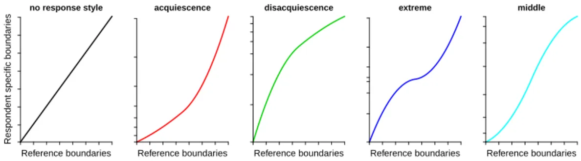
Response functions can be used to interpret the respondents’ response styles. Figure 2.3 shows examples of typical response functions corresponding to respondents who have no, acquiescence, disacquiescence (a tendency to disagree), midpoint, or extreme response styles.

(15)

no response style

Reference boundaries

Respondent specific boundaries

acquiescence

disacquiescence

extreme

middle

Figure 2.3: Response functions. The horizontal axis represents the reference boundary (scale), while the vertical axis represents the respondent-specific boundary.

2.3 Correcting and clustering preference data in the pres- ence of response style bias

Based on the ideas and definitions introduced in Section 2.2, we consider estimation of respondent-specific response functions. Moreover, we show that the estimated response functions can be used to correct for response style bias and, at the same time, to find clusters of respondents based on their corrected item preferences. In this paper, these response tendencies shown in Figure 2.3 are considered as response styles, and it is assumed that there are no respondents having response-style-like preference (e.g, there are no respondents whose true responses agree with all items). In addition, it is assumed that categories in all items to be applied to CCRS have the same direction (e.g., a category indicating “agree” has a high number in all items).

2.3.1 Modeling response functions

To estimate a response function, data that represent respondent-specific boundaries are required. Here, similar to dual scaling and CDS, we code the preference data as “rank- ordered boundary data”. This means that the indicated item preferences and the reference boundaries are converted to rank-orders for each respondent. The obtained boundary rankings reflect respondents’ tendencies to select certain rating categories.

Suppose that q scale preference data X = (x_ij) (i= 1, . . . , n;j = 1, . . . , m) are given with the reference boundaries b₁, b₂,· · ·b_q₋₁. Then, the rank-ordered boundary data f_iℓ, (ℓ= 1, . . . , q−1) can be obtained as follows.

f_iℓ=

m+q∑−1 t=1

(I{ξit< b_ℓ}+1

2I{ξit=b_ℓ})−1 2 where ξ_it=





b_ℓ+b_ℓ−1

2 (t= 1, . . . , m, xit=ℓ) bt−m (t=m+ 1, . . . , m+q−1)

(2.3.1) For t = 1, . . . , m, ξ_it indicate the representative values of a category, in our case, (b_ℓ + b_ℓ₋₁)/2. On the other hand, fort=m+ 1, . . . , m+q−1,ξ_itindicate reference boundaries.

(16)

b₁ b₂ b3 b₄ b5 b6

0123579

Rank ordered boundary data

υ1 t υ2

M₁ M₂ M₃

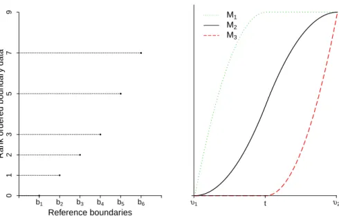
Figure 2.4: (Left) An example of rank-ordered boundary data. The horizontal axis corresponds to reference boundaries, the vertical axis shows f_iℓ values corresponding to each boundary. Each dot represents, f_i1, . . . , f_i6. (Right) Three I-spline basis functions.

I1,I2,I3 are shown with solid, dot and dashed line, respectively.

The same idea was used in CDS (constrained dual scaling) (Schoonees et al., 2015), in which the use of this idea followed from dual scaling for successive data (Nishisato, 1980).

To illustrate how this works in practice, consider 7-point scale preference data, xi = (5,6,7), is given. Using Equation (2.3.1), we obtainξi= (4.5,5.5,6.5,1,2,3,4,5,6), where ξi = (ξit),(t= 1, . . . , m+q−1). Then, sorting and converting these to rank-orders (starting from 0) yields

( )

ξ^sorted_i = 1 2 3 4 4.5 5 5.5 6 6.5

rank : 0 1 2 3 4 5 6 7 8

Sinceξ_i4 = 1,ξ_i5 = 2,ξ_i6 = 3,ξ_i7= 4,ξ_i8= 5,ξ_i9 = 6 corresponds to rank 0,1,2,3,5 and 7, respectively, we getf_i = (0,1,2,3,5,7). Figure 2.4 (left) plots thef_i= (f_iℓ) (ℓ= 1, . . . ,6) against these reference boundaries. Using this converted f_i, we see that respondent i demonstrates an acquiescence response style. For example, for f_i1, . . . , f_i4, the values increase one by one, which indicates that respondentidoes not select categories between the first and fourth reference boundaries frequently (i.e., the respondent does not often assign a rating smaller than 4). On the other hand, there is a large gap betweenf_i4 and f_i6, which indicates that categories between the fourth and sixth reference boundaries are often selected.

Usingf_iℓ, we consider a model for response functions corresponding to Definition 2.2.1, using I-Spline basis functions. Let ¯f_iℓ =f_iℓ/p, where p= m+q−1, so that ¯f_iℓ ∈[0,1].

(17)

Also, from here on, we useb_ℓ=ℓ/q, (ℓ= 1, . . . , q−1). In CCRS, ¯f_iℓis approximated as f¯iℓ≈ϕ^CCRS_i (ℓ/q), (i= 1, . . . , n;ℓ= 1, . . . , q−1)

where ϕ^CCRS_i (x) =

∑3 r=1

βirIr(x) s.t.

∑3 r=1

β_ir= 1, β_ir≥0 (r= 1,2,3)

(2.3.2)

Here,Ir (r = 1,2,3) are I-Spline basis functions, and βi1, βi2 and βi3 are the coeﬃcients ofI1,I2 and I3, respectively. I1,I2 and I3 are defined by

I1(x) =





2t(x−υ1)−(x²−υ²₁)

(t−υ1)² (υ₁ ≤x < t)

1 (t≤x≤υ2)

I2(x) =





(x−υ1)²

(t−υ1)(υ2−υ1) (υ₁ ≤x < t)

(t−υ1)

(υ2−υ1)+ ^2U(x_(υ⁻^υ¹⁾⁻^(x²⁻^t²⁾

2−t)(υ2−υ1) (t≤x≤υ₂)

(2.3.3)

I3(x) =





0 (υ₁ ≤x < t)

(x−t)²

(υ2−t)² (t≤x≤υ2)

and x ∈ [υ1, υ2], t = (υ1 +υ2)/2. Note that in this definition of I-spline functions, similar to Schoonees et al. (2015), we fix the number of order is 2, and use a single knot at the median of the given interval, as recommended by Ramsay (1988); Ramsay and Abrahamowicz (1989). For more general definition and its property, see, for example, Ramsay (1988).

In CCRS, we use υ1 = 0, υ2 = 1. Nonnegative conditions, βir ≥ 0 (r = 1,2,3), are required forϕi to be a monotone increasing function. See Section 2.3.5 for a more detailed justification of the rationale underlying the scaling of [υ₁, υ₂], f_iℓandb_ℓ to [0,1] as well as the advantages of adding the constraint∑₃

r=1β_ir = 1.

By using three I-spline basis functions (as shown in Figure 2.4, right), we can handle the five types of response styles shown in Figure 2.3. Further, in this model, only β_i1, β_i2 and β_i3 need to be considered to interpret the response styles. For example, a greater β_i3 value indicates a stronger tendency to select high categories because it results in more weight being placed on I3, which alters the shape of function to be more similar to the shape of the response function corresponding to the acquiescence response style (shown in Figure 2.3).

Now we can define a new correction method. Using the model defined in Equation (2.3.2), the response function can be estimated by “smoothing” via the constrained least squares method. In other words, given aq×1 vector ¯f_i = ( ¯f_iℓ) and a (q−1)×3 matrix, I= (Ir(ℓ/q)) (ℓ= 1, . . . , q−1 ; r = 1,2,3),β_i is obtained by minimizing

∑n i=1

∥f¯_i−Iβ_i∥², s.t.

∑3 r=1

β_ir = 1, β_ir ≥0 (2.3.4) where βi = (βi1, βi2, βi3). Using the estimated value of ˆβi, we can construct the “estimated” response function (see Definition 2.2.3), ˆϕ(x) = ∑₃

r=1βˆirIr(x). By transforming

(18)

all responses in the preference dataX using ˆϕ(x), we obtain a (n×m) “corrected data”

matrix, where response style bias is removed. Note that our new correction method can be considered as a special case of the framework introduced in Section 2.2.

In order to cluster respondents based on content in corrected data matrix, content-based clustering, such ask-means clustering, can be applied to the corrected data. We shall refer to this type of analysis as CCRS tandem.

Sequentially applying two methods (smoothing and clustering) may not yield optimal results for the correction and content-based clustering as the criteria of correction and clustering are optimized separately (e.g., Arabie, 1994). Therefore, we propose a method to conduct these two procedures simultaneously.

2.3.2 CCRS: Correcting and clustering response-style-biased data Simultaneous smoothing and clustering can be achieved by simply adding the two mini- mization criteria (e.g., Hwang, Dillon, & Takane, 2006). LetK be the number of content- based clusters. Then we define the objective function of CCRS as follows;

ψ(B,G,U|F¯,Z,I1,I2,I3) =λ

∑n i=1

∥f¯_i−Iβ_i∥²+ (1−λ)

∑n i=1

∑K k=1

u_ik∥Z_iIeβ_i−g_k∥²

(2.3.5) s.t.

∑3 r=1

β_ir = 1, β_ir ≥0 (r= 1,2,3 ;i= 1, . . . , n)

where B = (βi), G = (g_k), U = (u_ik), F¯ = (f¯i), (i = 1, . . . , n;k = 1, . . . , K), and, Z = (Zi), Zi = (z_ijℓ) (j = 1, . . . , m;ℓ= 1, . . . , q). The first term in equation (2.3.5) is the smoothing term, and the second term is the content-based clustering term. Note that λ∈[0,1] weighs these two terms and needs to be determined prior to the analysis.

In the content-based clustering term, k-means clustering is performed on the corrected data, namely, ZiIeβi = (ˆyij) (i = 1, . . . , n;j = 1, . . . , m). Specifically, the q×1 vector zij = (z_ijℓ) (ℓ = 1, . . . , q) is a dummy vector that takes z_ijℓ = 1 if respondent i selects category ℓ for the jth item; otherwise, z_ijℓ = 0. q ×3 matrix Ie = (Ir(τ(ℓ))) (ℓ = 1, . . . , q;r = 1,2,3) is a basis function matrix; however, unlike I, it takes the middle points of the boundaries as arguments to construct the corrected data in Definition 2.2.3.

The K×1 vector ui = (uik) (k = 1, . . . , K) is an indicator vector for the content-based cluster, whereuik = 1 if respondentibelongs to thekth content-based cluster; otherwise, uik = 0. Gis theK×m content-based cluster centroid matrix.

Choosing an appropriate value forλis a complicated task as there is no clear criterion that can be used. In Section 2.4, we show how diﬀerent values of λ aﬀect the clustering results and, in Section 2.5, we propose a pragmatic approach to determineλand Kat the same time.

Technically both CCRS and the correction method defined in Equation (2.3.4) can be applied to any ordinal categorical data, if the data are assumed to be contaminated by the eﬀect of response styles.

(19)

2.3.3 CCRS parameter estimation Algorithm to estimate CCRS parameters

To obtain parametersB,G,U, two operations, i.e., estimation of the response functions (estimation of B) and content-based clustering (estimation of Gand U), are performed sequentially. For fixed B, minimizing Equation (2.3.5) reduces to k-means clustering of the (response style corrected) data ZiIeβi (i = 1, . . . , n). On the other hand, when G and U are fixed, solving for B is less trivial as this appears in both terms in Equation (2.3.5). However, minimizing Equation (2.3.5) with respect to B can be reduced to a simple constrained least squares problem as follows;

Proposition 2.3.1. The objective function ofCCRS (2.3.5)can be written as follows.

ψ(B,G,U|F¯,Z,I1,I2,I3) =

∑n i=1

( √ λf¯i

(√

1−λ)G^′ui

)

−

( √ λI (√

1−λ)ZiIe )

βi

2

Proof.

ψ(B,G,U|F¯,Z,I1,I2,I3) =λ

∑n i=1

∥f¯i−Iβi∥²+ (1−λ)

∑n i=1

∑K k=1

uik∥ZiIβe i−gk∥²

=

∑n i=1

∥√

λ( ¯fi−Iβi)∥²+

∑n i=1

∑K k=1

uik∥√

1−λ(ZiIβe i−gk)∥² Note for any vectora^′= (a^′₁,a^′₂)^′,b^′ = (b^′₁,b^′₂)^′, it can be shown

∥a1−b1∥²+∥a2−b2∥² =

( a₁ a₂

)

− ( b₁

b₂ )

2

.

Using this andgk=G^′ui, the proposition can be verified immediately.

Using this property, parameters in CCRS are estimated based on the following algorithm.

Step 1: Initialization. Setλ and a convergence criterion ε, randomly choose an initial value forB,G,U, and set the number of iterationsw tow= 1.

Step 2: Response function estimation. For fixedG,U, updateBin such a way that Equation (2.3.1) is minimized with the constraint in Equation (2.3.2) (Haskell &

Hanson, 1981).

Step 3: Content-based clustering. For fixedB, update G,U using the following for- mula.

g_k=

∑_n

i=1uik(ZiIeβi)

∑_n

i=1u_ik u_ik=







1 (k= arg min

s∈{1,...,K}∥(√

1−λ(g_s−Z_iIeβ_i)∥² 0 (others)

(i= 1, . . . , n;k= 1, . . . , K)

(20)

Step 4: Convergence test Compute ψ^(w), the value of the objective function (2.3.5) using updated parameters and, forw >1, ifψ^(w)−ψ^(w⁻¹⁾ < ε, terminate; otherwise, letw=w+ 1 and return to Step 2.

Convergence of the algorithm is guaranteed because the objective function (2.3.5) is monotonically decreasing in subsequent steps. Note that in Step 1 of the algorithm, Ini- tial values forB,G,U need to be selected. This can be done randomly, e.g., by randomly generating values from uniform distribution. Alternatively, one could consider initial values forB,G,U by solving βi (i= 1, . . . , n) for the first term of Equation (2.3.5), that is, the optimal fitting of the response functions to the boundary data, and applyingk-means to corrected dataZiIβe i (i= 1, . . . , n) to obtain initial values forG,U. We shall refer to this type of initialization as CCRS tandem initialization.

Problem of local minimum in CCRS

In parameter estimation of CCRS, we apply k-means type algorithm, which is well- known for causing a serious local minimum problem. Though we proposed using “CCRS tandem initialization” above, this does not guarantees the global minimum. The commonly used approach to tackle with this problem is to run algorithm many times with diﬀerent randomly generated initial values, and select the estimates which yields the minimum value of objective function among estimates obtained by each run.

Figure 2.5 shows that the value of optimized CCRS objective function over the number of algorithm runs. Note that this is monotone non-increasing because the initial value is fixed at eachtth time (t= 1, . . . , T,;T = 1, . . . ,100 in this Figure). That is, for example, the 1st, 2nd and 3rd initial values are the same both when the number of initial values is 3 (T = 3 at the horizontal axis), and when the number of initial values is 10 (T = 10 at the horizontal axis).

This suggests that with λ= 0.2, the result of CCRS parameter estimation is unstable, because until around T = 40, the optimized value is frequently decreased. On the other hand, withλ= 0.8, the optimized value of CCRS objective function does not change over 100 runs, except the first three runs. That is, this figure suggests that in this case, the estimation result does not change whether the number of runs is 4 or 100. This should be because withλ= 0.2, the weight onk-means term is bigger than the smoothing term, and thus the estimation result tends to be unstable similarly tok-means algorithm.

2.3.4 Correcting preference data in the presence of response style bias by CDS

Schoonees et al. (2015) used constrained dual scaling (CDS) to estimate a response function defined similarly as in Section 2.2. In dual scaling, which is equivalent to correspondence analysis when analyzing contingency tables (van de Velden, 2000), category quantifications are obtained such that the quantifications best capture variance in the data in low dimensional space. For the analysis of preference data, dual scaling aims to

(21)

0 20 40 60 80 100

46485052

λ=0.2

The number of algorithm runs (T)

optimized value

0 20 40 60 80 100

24.3024.3424.3824.42

λ=0.8

The number of algorithm runs (T)

optimized value

Figure 2.5: The graph of optimized value of CCRS objective function over the number of algorithm runsT with diﬀerent initial values. That is, the horizontal axisT indicates how many times the algorithm runs with diﬀerent random initial values (t= 1, . . . , T), and the vertical axis indicates the minimum value of objective function among allT runs. In this numerical example, we fixed the initial values at thetth time of run for eacht= 1, . . . , T, for allT = 1, . . . ,100, so that the randomness of initial values can be removed to investigate the stability of the algorithm. The artificial data used in this numerical example are with n= 300,m= 10,D= 3,K = 3 andq = 5. How to generate the artificial data is explained in later Section 2.4.1.

(22)

quantify respondents, items and boundaries. In particular, in CDS, one-dimensional quantifications for respondents and boundaries are obtained to model monotonically increasing response functions for clusters of respondents. Response style bias can then be corrected for in a manner similar to that described in Section 2.2. A sequential analysis where we first correct for response style eﬀects using CDS, after which k-means is applied to the corrected data, can be seen as an alternative to the CCRS approach. We refer to such an approach as CDS tandem analysis.

As CDS is based on dual scaling, there are several restrictions. To explain this in detail, letviand wdℓdenote quantified values by CDS for respondenti, and theℓth boundary for thedth response-style-based cluster (d= 1, . . . , D), respectively. In addition, suppose that a respondenti belongs to the dth response-style-based cluster. In CDS, wdℓ = ϕ^CDS_d (ℓ), whereϕ^CDS_d is the CDS response function for thedth response-style-based cluster. Then, ϕ^CDS_d approximates the rank ordered boundary datafiℓ as

f˜_iℓ≈v_iϕ^CDS_d (ℓ), (i= 1, . . . , n;ℓ= 1, . . . , q−1) (2.3.6) where ϕ^CDS_d (x) =µ_d+

∑3 r=1

α_drIr(x) s.t. α_dr ≥0, (r = 1,2,3)

and ˜f_iℓ=f_iℓ−p/2, wherep=m+q−1. For the spline basis functionIr in CDS,υ₁ and υ₂ are set to 0 and q (rather than 0 and 1 as is the case in CCRS) respectively. For more details, see Schoonees et al. (2015).

Comparing Equation (2.3.6) with Equation (2.3.2), it is clear that CDS only estimates response functions for response-style-based clusters d = 1, . . . , D. Hence, due to the one-dimensional approximation only one parameter v_i (i= 1, . . . , n) in Equation (2.3.6) is respondent-specific. Therefore, estimating response functions in CDS could incur a significant loss of respondent-specific information.

Note that, by setting D = n and fixing the cluster indicator, CDS may be used to estimate respondent-specific α_d (d= 1, . . . , n) values. However, in practice, this process only yields degenerate solutions in which the parameters are zero or close to zero due to the one-dimensional reduction.

2.3.5 Properties and interpretation of CCRS

In addition to yielding content based clusters, CCRS can provide several insights into response styles. In particular, the constraint,∑₃

r=1β_ir = 1, the lack of a constant term, and the scaling of the range of f_iℓ and boundaries b_ℓ to [0,1] are useful for two reasons:

first, these constraints restrict the corrected data to [0,1] for all respondents and items.

Second, these constraints facilitate a straightforward visualization of response styles.

(23)

The range of corrected data Proposition 2.3.2. Let

ϕi(x) =

∑3 r=1

βirIr(x), x∈[0,1]

where βir ≥0 (r= 1,2,3 ; i= 1, . . . , n)

be a monotone response function of respondent i. Imposing the constraint ∑₃

r=1βir = 1 is equivalent to imposing

ϕi(0) = 0, ϕi(1) = 1.

Equivalently,

ˆ

yij ∈[0,1]

where Z_iIeβ_i= (ˆy_ij) (i= 1, . . . , n;j = 1, . . . , m)

Proof. The proposition follows immediately from Equation (2.3.3) by settingυ₁= 0 and υ₂ = 1.

In other words, the constraint∑₃

r=1β_ir = 1 implies a constraint on the range ofϕ_i, and, as a result, a constraint on the range of the corrected data, ˆy_ij. This is useful for avoiding excessive values for β_ir. If respondent i could receive a very large β_ir for some r, the corrected data ˆy_ij (j= 1, . . . , m) would also become quite big, and as a result, respondent iwould be considered as an outlier in the cluster analysis. However, large values forβ_ir do not necessarily indicate that a respondentiis an outlier with respect to item preferences, even though the observation could be considered to be an outlier with respect to response styles. Thus, the summation constraints prevents the corrected values to be aﬀected by strong response style eﬀects.

Visualization of response styles

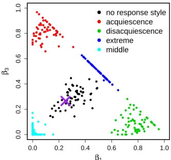
Constraining βir(r = 1,2,3) to a sum of 1 allows for a simple visualization of these coeﬃcients. Such a visualization can be used to interpret the respondent-specific response tendencies. In particular, by combining a scatterplot of the respondent-specific estimates of βi1 against βi3, we obtain a visualization of the estimated response functions. Figure 2.6 illustrates this for an example dataset. Note that respondents having no response style (Definition 2.2.2) can be expressed as the single cross point in this plot, as indicated in the following proposition.

Proposition 2.3.3. Let

ϕ_i(x) =

∑3 r=1

β_irIr(x), x∈[0,1]

be the true response function of respondenti, and supposeβir ≥0 (r = 1,2,3), ∑₃

r=1βir = 1. Then respondent ihas no response style, if and only if

βi1 =βi3= 0.25, βi2 = 0.5.

(24)

Proof. First, we show that having no response style =⇒βi1=βi3 = 0.25. From Definition 2.2.2, having no response style means having the identity function as response function.

In that case,

∂²

∂x²ϕi(x) = 0.

On the other hand, when υ₁= 0 and υ₂= 1, from Equation (2.3.3) it follows that

∂²

∂x²ϕ_i(x) =





−8β1+ 4β2 (0≤x <1/2)

−4β₂+ 8β₃ (1/2≤x≤1)

Therefore having no response style implies β₁ = 2β₂ for 0 ≤x < 1/2, and β₃ = 2β₂ for 1/2≤x≤1. Since β_ir(r = 1,2,3) is common for all x∈[0,1],

2βi1 =βi2 = 2βi3. From the constraint∑₃

r=1β_ir = 1, the result immediately follows.

Next, to proof that β_i1 = β_i3 = 0.25 =⇒ having no response style, note that from the constraint ∑₃

r=1β_ir = 1 it immediately follows that β_i2 = 0.5. Then, substituting β_i1 =β_i3= 0.25 and β_i2= 0.5 into Equation (2.3.2) yields

∂

∂xϕ_i(x) = 1, ∂²

∂x²ϕ_i(x) = 0, x∈[0,1].

Hence,ϕi(x) is an identity function. □

From this proposition, it follows that the purple cross in Figure 2.6, with coordinates (0.25,0.25), corresponds to no response style. The black points close to this purple point also correspond to respondents who do not have clear response style and deviations from this point indicate the presence of response styles.

2.4 Simulation study of CCRS

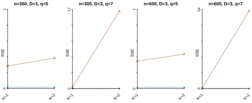
We conducted a simulation study to evaluate the performance of CCRS. In this simulation study, we investigated two things:

• the accuracy of correction comparing our CCRS correction defined in Equation (2.3.4) with CDS correction.

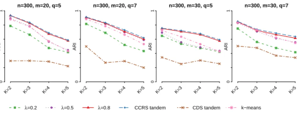
• the accuracy of content-based clustering comparing our CCRS in Equation (2.3.5) withk-means and CDS tandem.

Note that in CDS tandem, preference data are first corrected using CDS. Then,k-means is applied to the corrected data.

To assess the performance of the methods, we consider two scenarios. In scenario I, we assume that there are two kinds of underlying clustering structures: content and response- style-based clusters. In scenario II, only an content-based clustering structure is assumed.

By considering these two scenarios, data are generated corresponding to situations that are assumed to underlie, either implicitly or explicitly, both the CDS and the CCRS methods.

(25)

0.0 0.2 0.4 0.6 0.8 1.0

0.00.20.40.60.81.0

β1

β3

×

no response style acquiescence disacquiescence extreme

middle

Figure 2.6: A scatterplot of βi1 and βi3 for each respondent (i= 1, . . . , n) estimated by CCRS using λ= 0.8 for a simulated data set with n= 300, m = 20, K = 2, q = 7. The colors correspond to the true response styles. The way to generate these data is explained in Section 2.4.

2.4.1 Data generation

The data generation process can be divided into two steps: (i) generation of true pref- erencesx^∗_ij ∈Rand (ii) mapping of the true preferences to q scale data x_ij ∈ {1, . . . , q}. Content-based clusters and, for scenario I only, response-style-based clusters, are induced in steps (i) and (ii), respectively.

(i) Generation of the true preferences

As we want a subset of items to be related to the clustering structure, the m items are divided into two groups: items related to the clustering structure and “noisy” items that are unrelated to the clusters.

In addition, the cluster-related items are divided further into three groups with diﬀerent means of true preferences to ensure that the content-based clusters do not resemble either of the response-style-based clusters shown in Figure 2.7 (left). To see why this is useful, consider a situation in which all cluster-related items have one common cluster center.

The corresponding content-based cluster could then be considered a response-style-based cluster corresponding to acquiescence, disacquiescence, or midpoint depending on the mean (e.g., if the means for all cluster-related items are high, it could be seen as an acquiescence response-style-based cluster). Furthermore, if all items have two centers only, the resulting cluster could be considered a response-style-based cluster corresponding to the extreme response style (e.g., if the means for the two item groups is extremely either high or low).

Thus, both possibilities are avoided by dividing the cluster-related items into three groups