JAIST Repository
https://dspace.jaist.ac.jp/
Title 量子計算の複雑さに関する研究
Author(s) 三原, 孝志
Citation
Issue Date 1997‑03
Type Thesis or Dissertation Text version author
URL http://hdl.handle.net/10119/832 Rights
Description Supervisor:國藤 進, 情報科学研究科, 博士
By Takashi Mihara
A thesis submitted to
School of Information Science,
Japan Advanced Institute of Science and Technology,
in partial fulllment of the requirements
for the degree of
Doctor of Information Science
Graduate Program in Information Science
Written under the direction of
Professor Susumu Kunifuji
January 1997
Copyright c 1997 by Takashi Mihara
Nowadays, there are many problems that are intractable to b e solved on ordinary
computers. Therefore,inordertoinventmorep owerfulcomputers,weneedacomputing
model that is based on quantum physics, i.e., a quantum computer, because the com-
putational principles of ordinary computers are based on classicalphysics,whereas the
principles of the real worldcan be explainedby quantum physics. In 1985, for the rst
time,Deutschproposeda computingmodelinvolvingasuperp osition of physicalstates,
which is one of inherent properties of quantum physics, as a quantum Turing machine
(QTM)andin1993,Bernsteinand VaziranimathematicallyformalizedtheQTM.After
that, some results have indicated that the QTM may be more powerful than ordinary
computers. In 1994, in fact, Shor showed that the QTM can nd discrete logarithms
andfactor integersinpolynomialtimewith boundederrorprobability. Wedonotknow
whether ordinary computers can eciently solve these problems or not. In this thesis,
we present an overview on quantum computers and quantum complexity classes and
then, we showsome results onthe complexity and algorithms based onthe QTM.
Some techniques for solving problems eciently on QTMs have been proposed. Es-
pecially, the most well-known techniques, aquantumFouriertransformand a quantum
iterating method, have been used. A quantum Fourier transform is a quantum ver-
sion of discrete Fourier transforms and can eciently obtain some properties of func-
tions. By this technique,weshow that the perio ds in some kindsof periodic functions,
f(x) = f(x+r) and x = f r
(x) for a period r, can b e found in polynomial time with
boundederrorprobabilityonQTMs. Some ofthefunctionsproposedaspseudo-random
generators are also included inthese functions.
Aquantumiteratingmethodisamethodtoincreasetheprobabilityofacceptingstates
byusinganalgorithmrep eatedly. Bythistechnique,weshowthatforanunsortedtable
T of n items and a query item q, there is aquantum searchalgorithm that nds apair
of indices(j;k)correspondingto twosuccessiveitems, T[j]and T[k], whichsatisfythat
T[j] qT[k], in expected time O(n 1=2
)with boundederror probability. As aspecial
case,this algorithmcan nd theminimumorthe maximumvalueof T inexpectedtime
O(n 1=2
) with bounded error probability. Moreover, we also showthat QTMs can solve
some problems incomputational geometrymore eciently than ordinary computers.
Finally, we investigatethe relationships between the computational complexity and
quantum physics. Although NP-complete problems appear inmany situations, nobo dy
knows whether ordinary computers can eciently solve these problems or not. On the
other hand, the problem of measurement is one of the most interesting problems in
physics and nobody can explain suciently what happens when we measureyet. Here,
we propose the following two assumptions on measurement: (i) Assumption 5
1 : a
superpositionof physicalstates is preservedaftermeasurements and allof the states in
the superposition can be measured in time proportional to the numb er of the states in
the superposition, and (ii) Assumption 5
2
: we can measure the existence of a specic
physicalstate C in a given superp osition with certainty in polynomialtime if the state
C exists in the superposition. Then, we show that there is a QTM that solves the
satisabilityproblem (SAT)in O (2 ) timeunder Assumption 5
1
and there isa QTM
thatsolvesSATinn O (1)
timeunderAssumption 5
2
,wheren isthelengthofaninstance
of SAT. SATisa typicalNP-complete problem.
In the course of conducting this research, the authorwas fortunateto receiveguid-
ances and encouragementsfroma large numb erof p eople. Withoutthem, this research
would have never been accomplished. To begin with, the rst and most important
person to whom the author would like to express his sincere gratitude is his principal
advisor Professor Susumu Kunifuji of Japan Advanced Institute of Science and Tech-
nology (JAIST). He gave the author his constant encouragements and kind guidances
duringthis research.
TheauthorwouldliketothankhisadvisorAssociateProfessorSatoshiTojoofJAIST
for his helpful discussions and suggestions. The author also would like to thank to
Professor Hiroakira Onoand Professor Eiji OkamotoofJAIST for their kindcomments
and suggestions.
Theauthorisgratefultoallwhohaveaectedorsuggested hisareasofresearch. As-
sociate ProfessorTetsuroNishino ofthe Universityof Electro-Communications inspired
the author through his constant activities on quantum computer, and gave the author
valuable commentsand continuous encouragements.
The author is grateful to allwho have read the manuscript and oered useful com-
ments: Dr. ThanarukTheeramunkong, Dr. MasahiroMamb o, Dr. Ratana Rujiravanit,
KeisukeTanaka, Shao-ChinSung, and HiroyukiShirasu.
The author devotes his sincere thanks and appreciation to all of them, and his col-
leagues.
1 Intro duction 1
2 Preliminaries 5
2.1 Notations : : : : : : : : : : : : : : : : : : : : : : : : : : : : : : : : : : : 5
2.2 Turing Machines : : : : : : : : : : : : : : : : : : : : : : : : : : : : : : : 5
2.3 Reversible Computation : : : : : : : : : : : : : : : : : : : : : : : : : : : 7
3 Quantum Computers 12
3.1 Quantum Computers b efore Deutsch's : : : : : : : : : : : : : : : : : : : 12
3.1.1 SimulatingTMs by QuantumPhysics : : : : : : : : : : : : : : : : 12
3.1.2 Feynman'sUniversal Quantum Simulator: : : : : : : : : : : : : : 13
3.2 Quantum Turing Machine : : : : : : : : : : : : : : : : : : : : : : : : : : 13
3.2.1 Denitionof Quantum Turing Machine : : : : : : : : : : : : : : : 13
3.2.2 PhysicalRepresentation of QTM : : : : : : : : : : : : : : : : : : 15
3.3 OtherQuantum ComputingModels : : : : : : : : : : : : : : : : : : : : : 17
3.3.1 QuantumCircuits: : : : : : : : : : : : : : : : : : : : : : : : : : : 17
3.3.2 QuantumCellular Automata: : : : : : : : : : : : : : : : : : : : : 18
3.4 Realizabilitiesof QuantumComputers : : : : : : : : : : : : : : : : : : : 20
4 Quantum Complexity Classes 22
4.1 OrdinaryComplexity Classes : : : : : : : : : : : : : : : : : : : : : : : : 22
4.1.1 Complexity Classes BasedonTMs : : : : : : : : : : : : : : : : : 22
4.1.2 Complexity Classes BasedonPTMs: : : : : : : : : : : : : : : : : 22
4.1.3 Reducibilityand Completeness : : : : : : : : : : : : : : : : : : : 24
4.2 Quantum Complexity Classes and Relationships Between Classes : : : : 24
4.2.1 BQP : : : : : : : : : : : : : : : : : : : : : : : : : : : : : : : : : : 25
4.2.2 OtherQuantum Complexity Classes: : : : : : : : : : : : : : : : : 28
4.2.3 RelationshipsBetweenComplexity Classes : : : : : : : : : : : : : 29
5 Perio dic Functions 32
5.1 Intro duction : : : : : : : : : : : : : : : : : : : : : : : : : : : : : : : : : : 32
5.2 Quantum Fourier Transforms : : : : : : : : : : : : : : : : : : : : : : : : 32
5.2.1 Shor'sQuantum Algorithmfor Factoring Integers : : : : : : : : : 32
5.2.2 VariousTransforms : : : : : : : : : : : : : : : : : : : : : : : : : : 34
5.3.1 Typ e f(x)=f(x+r): : : : : : : : : : : : : : : : : : : : : : : : : 39
5.3.2 Typ e x=f r
(x) : : : : : : : : : : : : : : : : : : : : : : : : : : : : 41
6 Quantum Search Algorithms 44
6.1 Intro duction : : : : : : : : : : : : : : : : : : : : : : : : : : : : : : : : : : 44
6.2 Search Algorithms onQTMs : : : : : : : : : : : : : : : : : : : : : : : : : 44
6.2.1 Grover's Quantum SearchAlgorithm : : : : : : : : : : : : : : : : 44
6.2.2 ExtendedQuantum SearchAlgorithm: : : : : : : : : : : : : : : : 46
6.3 Applications : : : : : : : : : : : : : : : : : : : : : : : : : : : : : : : : : : 49
7 The Complexity of NP-complete Problems 52
7.1 Intro duction : : : : : : : : : : : : : : : : : : : : : : : : : : : : : : : : : : 52
7.2 Solving SATunder the First Assumption : : : : : : : : : : : : : : : : : : 53
7.3 Solving SATunder the Second Assumption : : : : : : : : : : : : : : : : : 58
8 Conclusions 63
A Quantum Theory 65
A.1 Hilbert Spaces : : : : : : : : : : : : : : : : : : : : : : : : : : : : : : : : : 65
A.2 Tensor Products: : : : : : : : : : : : : : : : : : : : : : : : : : : : : : : : 67
A.3 Unitary Operators : : : : : : : : : : : : : : : : : : : : : : : : : : : : : : 68
A.4 Quantum Physics : : : : : : : : : : : : : : : : : : : : : : : : : : : : : : : 70
Bibliography 71
Publications 80
2.1 A Turing machine. : : : : : : : : : : : : : : : : : : : : : : : : : : : : : : 6
3.1 A Tooligate. : : : : : : : : : : : : : : : : : : : : : : : : : : : : : : : : : 17
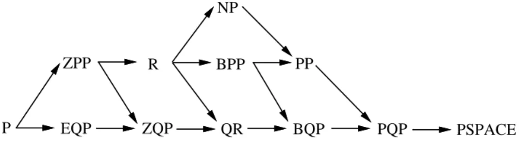
4.1 Relationshipsbetween complexityclasses.: : : : : : : : : : : : : : : : : : 31
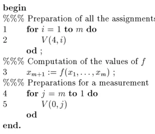
7.1 The QTM U. : : : : : : : : : : : : : : : : : : : : : : : : : : : : : : : : : 54
7.2 The program that the QTM U executes under Assumption 5
1
. : : : : : : 55
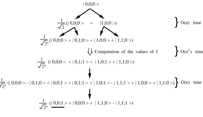
7.3 The computationexecuted by the QTM U. : : : : : : : : : : : : : : : : : 57
7.4 The program that the QTM U executes under Assumption 5
2
. : : : : : : 58
7.5 The changes of the superpositionof congurations ofthe QTM U. : : : : 62
2.1 A reversible computingprocess. : : : : : : : : : : : : : : : : : : : : : : : 11
Introduction
A standard theoretical model of computing devices is a Turing machine that was pro-
posedbyTuringin1930's. Forsomespecicproblems,theabilitiesofordinarycomputers
aremore p owerfulthanthoseofhumanbeings. Onthe otherhand, manyproblemsthat
areintractabletobesolvedonordinarycomputersarealreadyknown. Furthermore,the
computational principles of ordinary computers are based onclassical physics, whereas
itisthoughtthat the principles ofthe real worldcan beexplained by quantum physics.
Namely, it is well-known that classicalphysicsis sucient to explain macroscopic phe-
nomena but is not sucient to explain microscopic phenomena like the interference of
electrons. In these days,the speed-upand down-sizing of computing devices have been
carriedout byusing quantum physicaleects, however,the computational principles of
these devices are based onclassical physics.
In this situation, from 1980's, physicists have seen the limitations of ordinary com-
puters when they simulated physical phenomena on those computers. They thought
that, since the current computational principles are based on classical physics, they
might b e able to make a more p owerful computer if they could use the computational
principlesbasedonquantumphysics,whichcanexplaintherealworldmoreprecisethan
classical physics. Thus, they proposed a computer that involves inherent properties of
quantum physics asthe computational principlesand called ita quantum computer.
In early models of quantum computers, researchers placed a great importance on
nding precise representations of Turing machines based on quantum physics(e.g., see
[9,11, 14, 93]). Thus,inherentpropertiesofquantumphysicswerenotinvolvedinthose
models. Inother words,theirpurposewastodesigngoodsimulatorsofTuringmachines
by using quantumphysics.
On the other hand, Feynman and Deutsch prop osed the mo dels of quantum com-
puters in which inherent properties of quantum physics are involved. In 1982, Feyn-
man asked whether ordinary computers can eciently simulate physical phenomena
and pointed out that they may not be able to eciently simulate physical phenomena
[54]. Moreover, he suggested that a new computer based on quantum physics, a quan-
tum computer, may be more powerful than ordinary computers. However, he did not
formalizehis quantumcomputer.
quantum physics are involved was proposed as a quantum Turing machine (QTM) by
Deutsch [39]. However, Deutsch's quantum computer was not suciently formalized.
So,hedidnot preciselyevaluatethecomputingpowerofhisquantumcomputeranddid
notmentionanythingaboutthecomputationalcomplexityofhisquantumcomputation.
In 1993, Bernstein and Vaziranimathematicallyformalized the QTM [23] and some
resultshaveindicatedthattheQTMseemstobemorepowerfulthanordinarycomputers
(e.g.,see[22,24,25, 41,68, 113]). In1994,infact,Shorshowedthatdiscretelogarithms
andfactoring integersare included inBQP,whichisa languagethat can beaccepted in
polynomial time with bounded error probability on QTMs [108, 110]. These problems
are generally considered hard on ordinary computers and have b een used as the bases
of several prop osedcryptosystems.
Many physicists are also studying physical realizabilities of the QTM, and Lloyd
reportedthat the QTM is p otentiallyrealizable [77, 78]. On the otherhand, fromcom-
puterscienticpointsofview,itis almostimp ossible toconstructa newsimulatorfor a
QTMwheneveritsnitecontrolischanged. Thus,itisimportanttoanswerthequestion
whether a universal QTM exists. Deutsch showed that there is a universal QTM [39].
However, if weuse his construction, the simulatingoverhead can be exp onentialin the
runningtime of the simulated QTM inthe worst case. After that, Bernstein and Vazi-
rani showed that there is a universal QTM whose simulating overhead is p olynomially
bounded[23].
The remainder of this thesis is divided into six major chapters. In Chapter 2, we
describe elementary denitions and notations. We dene Turing machines that are
standard theoreticalmodels ofcomputing devices. Thereare alot of computingmodels
that are known as Turing machines. Here, we dene only two typical Turing machines,
a deterministic Turing machine and a nondeterministic Turing machine. A QTM is
dened based on these models. Since the execution of the QTM is evolved by unitary
matrices, it is also a mo del of reversible computation. Therefore, in this chapter, we
alsodescribethedenitionofareversibleTuringmachinethatwasproposedbyBennett
[15].
InChapter3,wereviewseveralmodelsofquantumcomputers. Aquantumcomputer
was rstly proposed as a QTM by Deutsch [39]. His quantum computer, for the rst
time, involves inherent prop erties of quantum physics as the computational principles.
Nowadays,many computer scientists studythe complexityand algorithms based onhis
model. However, since there are other quantum computing mo dels such as quantum
circuits and quantum cellularautomata, we also describe these models briey. Finally,
we summarize the realizabilitiesof quantumcomputers.
InChapter4,wedenetypicalcomplexityclassesbasedonordinaryTuringmachines
and complexityclasses basedon QTMs. QTMs can be regardas akind of probabilistic
Turing machines, because in quantum physics we can obtain results only probabilisti-
cally. Therefore,wedene complexity classes based on QTMs as classes corresponding
to the probabilistic complexity classes and call the complexity classes based on QTMs
quantum complexity classes [23, 83]. Moreover,we also show the relationships between
In Chapter 5, we discuss metho ds to nd the periods of functions eciently. Shor
showedthataQTMcannddiscretelogarithmsandfactorintegerseciently[108,110].
No polynomial time algorithm to nd these problems on ordinary computers is known.
In order tosolvethese problems eciently, hereduced themto the problems of nding
the p eriodsof somefunctions and used themost famous technique forsolving problems
eciently onQTMs, a quantum Fourier transform.
We show that the periods in some kinds of periodic functions,f(x)=f(x+r) and
x=f r
(x)foraperio dr,canbefoundinpolynomialtimewithboundederrorprobability
onQTMs byusing the quantumFouriertransform[84]. Forinstance, wecan eciently
solve a cycle problem on a QTM. Given a nite domain D, let us consider a function
f :D!D suchthat ithas s+r distinctvaluesx
0
=f 0
(x
0 );f
1
(x
0
);...;f s+r 01
(x
0 ),but
f s
(x
0 ) = f
s+r
(x
0
). This means that f j
(x
0 ) = f
j+r
(x
0
) for all j s. A cycle problem
forf and x
0
isto nd the pair (s;r). Sedgewicket al. showedthat ordinarycomputers
need O(n) time in order to solve the problem, where n =s+r [106]. We show that a
QTMcansolveitin(log
2 n)
O (1)
time. Someofthefunctionsprop osedaspseudo-random
generators are also included inthese functions.
In Chapter 6, we discuss quantum search algorithms for a table search (e.g., a
database search). In order to eciently search items in a table on a QTM, we use an-
other well-known technique, a quantum iterating method. A quantum iterating method
wasproposed byGroverand is amethodtoincrease the probabilityof accepting states
by using analgorithm repeatedly. He showedthat for anunsorted table T of n distinct
items,T[0];T[1];...;T[n01], thereis aquantumsearchalgorithm that nds the index
m of a query item q(=T[m]) in expected time O(n 1=2
) with b ounded error probability
[60]. Ordinary computersneed O(n) time to nd the index.
We show that for an unsorted table T of n items and a query item q (where q may
not necessarily exist in T), there is a quantum search algorithm that nds a pair of
indices (j ;k) corresponding to two successive items, T[j] and T[k], which satisfy that
T[j] qT[k],inexp ectedtimeO (n 1=2
)withboundederrorprobability. Ouralgorithm
uses Grover's search algorithm as a subroutine, and as a special case, we can nd the
minimum orthe maximum valueof T by using this algorithmin expected time O(n 1=2
)
with b ounded error probability. Moreover, we also show that QTMs can solve some
problems incomputational geometrymore ecientlythan ordinary computers.
In Chapter 7, we discuss methods to solve NP-complete problems on QTMs. Al-
though NP-complete problems appear in many situations, nobody knows whether or-
dinary computers can eciently solve these problems or not. It is one of the most
importantissues intheoreticalcomputer sciencetond ametho d tosolveNP-complete
problems eciently.
Even if a QTM can compute all the values of a function by using quantum parallel
computation,wecannot,ingeneral,obtainallthe valuesofthe functionsimultaneously.
Moreover, according to current quantum physics, it is not certain whether we can e-
ciently read each value in the obtained superposition. These are b ecause the following
measurement problem has not been completely solved.
What will happenwhen we measurea quantum physicalobject ?
Explain it in termsof quantum physics.
Therefore, we study the relationships between the assumptions on measurement and
the eciency of quantumcomputation. Especially, we study the satisability problem
(SAT), because SAT is a typical NP-complete problem [56]. Here, we propose the
following two assumptions on measurement: (i) Assumption 5
1
: a sup erposition of
physicalstatesispreservedaftermeasurementsand allofthe statesinthe superposition
can b e measured intime proportional tothe numb er of the states in the superposition,
and (ii) Assumption 5
2
: we can measure the existence of a specic physical state C
in a given superp osition with certainty in polynomial time if the state C exists in the
superposition. Consequently,weshowthataQTMcansolveSATinO(2 n=4
)time under
Assumption 5
1
and a QTM can solve SAT in n O (1)
time under Assumption 5
2
, where
n is the length of aninstance ofSAT [81, 82].
The assumptions aboveare not widely supported in current quantum physics, how-
ever,nobo dy knowswhether these assumptions are valid or not. This is b ecause inter-
pretationsof measurement havenot been xedyetamongphysicists. Themeasurement
problem is one of the central issues in quantum physics and several interpretations of
measurementexist. Inthissituation,itisimp ortanttondvariousrelationshipsbetween
the restrictions onmeasurementand the eciencyof quantumcomputation.
Preliminaries
2.1 Notations
In this section,wedescribesome notations that are used inthis thesis.
1. The Sets
C : the setof complex numb ers.
R : the setof real numb ers.
Z : the setof integers.
Z +
: the set ofpositiveintegers.
Z
n
: f0;1;...;n01g.
N : the setof natural numb ers
2. O-notation
O(f) is the set of functions g such that for some constant c> 0 and for all
but nitely many n, g(n)<cf(n).
(f) is the set of functions g such that for some constant c > 0 and for
innitely many n, g(n)>cf(n).
2(f)is the set of functionsg suchthat for some constants c
1
;c
2
>0and for
all but nitely many n, c
1
f(n)<g(n)<c
2 f(n).
2.2 Turing Machines
A Turing machine isa kindof mathematical computingmachine model. The denition
of a Turing machine is described in this section. For a more complete overview, the
reader is referred to [3, 61, 91]. There are a lot of computing models that are known
asTuringmachines. Here, we denoteonlytwo typical Turing machines,a deterministic
Turing machine and anondeterministic Turingmachine.
. . . . . . 2 i
. . . 1 A tape
A finite control
A tape head
a a a
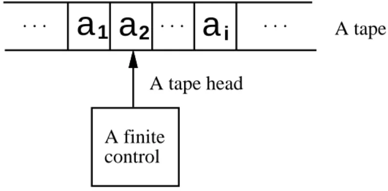
Figure 2.1: A Turing machine.
As shown in Fig. 2.1, a deterministic Turing machine consists of a nite control,
an innitetape, and a tap e head. In one move, the Turingmachine, depending on the
symb ol scannedby the tapehead and the state of the nite control,
1. changes state,
2. writes asymbol on the tapecell scanned, replacing what was writtenthere, and
3. movesits headleft one cell, right one cell, or keepitstationary.
Denition 2.1 . A deterministic Turing machine(DTM) is a 7-tuple
M =(Q;6;0;;q
0
;b;F), where
Q is the nite set of states,
0 is the nite set of tape symbols,
b20 is a blank symbol,
60 isthe set of input symbols,
is the state transition function that is a mapping from Q20 to Q202
f0;0;+g,
q
0
2Q isthe initial state,
F Q isthe set of nal states.
Here, f0;0;+g in the state transition function decidesthe movement of its head, i.e.,
0(resp. 0, +) means the movement of its head left one cell (resp. stationary, right one
cell).
AnondeterministicTuringMachine(NDTM)consistsofa7-tupleM =(Q;6;0;;q
0
;B;F)
whereallcomponentshavethe same denitionas the DTM,except that the statetran-
sition function is a mapping from Q20 to subsets of Q202f0;0;+g. Here, we
dened only one-tap e Turing machines, however, we can also dene many-tap e Turing
machines. Furthermore,auniversalTuringmachineisdenedasaTuringmachinethat
can simulate any Turing machine with any input.
provethat a Turingmachine is equivalent toour intuitivenotion of computation, how-
ever,therearemanyargumentsforthisequivalence,whichhasbecomeknownasChurch-
Turing thesis.
Church-Turing Thesis:
The intuitivenotionof computable function can b eidentied with
the class of computationwith a Turing machine.
Therefore,aTuringmachineisequivalenttoallofthemostgeneralmathematicalnotions
ofcomputation. Furthermore,DeutschreinterpretedtheChurch-Turingthesisphysically
fromaviewpointof constructingareal computerand calleditChurch-Turing principle.
That is,a quantum computer is a computing model prop osedunder this interpretation
(cf. Chapter 3).
2.3 Reversible Computation
Foralongtime,acomputationwasthoughtasanirreversibleprocess. However,Bennett
constructed a logical reversible Turing machine and showed that the reversible Turing
machine can simulate an irreversible computation with constant slowdown [15, 16, 17,
18, 76].
AsshowninSection2.2, thestatetransitionfunctionofaone-tap eTuringmachine
can b e represented by the following quintuple.
At!A 0
t 0
; (2.1)
where
A and A 0
are the statesbeforeand after the transition, resp ectively,
t is the tap e symb olthat is read atthe head position,
t 0
is the tap e symb ol thatwill be writtenat the head position, and
is the movementof the head (i.e., 2f0;0;+g).
A Turing machineis deterministicif and only if itsquintuples havenon-overlapping
domains,andisreversibleifandonlyiftheyhavenon-overlappingranges. Itwasthought
that a computation can be executed only irreversibly because the ranges of quintuples
overlap. Therefore,ausual Turingmachine is not reversible. However,Bennett showed
thatareversiblecomputationcanbeexecutedwithsplittingthestatetransitionfunction
into a read-write operation and a head movement operation, and a reversible Turing
machine can simulate an irreversible computation with constant slowdown. Here, we
denoteBennett's construction of areversible Turing machine(reversibleTM) [15].
First, wedene the following quadruplefor areversibleTM that corresponds tothe
usual state transition function.
dened by
A[t
1
;t
2
;...;t
n ]!A
0
[t 0
1
;t 0
2
;...;t 0
n
]; (2.2)
where
A and A 0
are the states before and after the transition, respectively,
t
k
isthe tape symbol thatisread onthe kth tapeor = (indicatingthatthe kth
tape is not read during the transition), and
t 0
k
isthe tape symbol that will be written on the kth tape or the movementof
the kth head (i.e.,
k
2f0;0;+g).
Notethat ausualTuringmachineexecutesthe read-writeoperationand theheadmove-
ment operation at the same time, on the other hand, the reversible TM writes on the
tapeif and only if it has just read it, and movesthe tapehead if and only if it has not
just read it. Thus, the following quadruplesdene the mappings of the whole-machine
statesthatare one-to-one. Anyread-write-movementquintuplecanbesplit intoaread-
write operation and a head movementoperation. Therefore, the quintupleof Eq. (2.1)
is equivalent toa pair of quadruples.
A[t
1
;t
2
;...;t
n
] ! A"[t 0
1
;t 0
2
;...;t 0
n
]; and
A"[=;=;...;=] ! A 0
[
1
;
2
;...;
n ];
whereA"isanewstatedierentfromAandA 0
. When several quintuplesaresosplit, a
dierentconnectingstateA" mustbeused foreachtoavoidintro ducing indeterminacy.
Now,letus considerthe following two n-tape quadruplesof Eq. (2.2).
A[t
1
;111;t
n ]!A
0
[t 0
1
;111;t 0
n
]; (2.3)
and
B[u
1
;111;u
n ]!B
0
[u 0
1
;111;u 0
n
]: (2.4)
Theyhave the followingadditional important prop erties:
1. Eqs. (2.3) and (2.4) are mutually inverse if and only if
(A=B 0
)^(B =A 0
)
^(8k((t
k
=u
k
==)^(t 0
k
=0u 0
k )_(t
k
6==)^(t 0
k
=u
k )^(t
k
=u 0
k ))):
2. The domainsof Eqs. (2.3) and (2.4) overlap if and only if
(A=B)^(8k((t
k
==)_(u
k
==)_(t
k
=u
k ))):
3. The rangeof Eqs. (2.3) and (2.4) overlapif and onlyif
(A =B )^(8k((t
k
==)_(u
k
==)_(t
k
=u
k ))):
Thus, an n-tape reversible deterministic Turing machine is dened as a nite set of
n-tape quadruplesof Eq. (2.2), notwoof which overlap eitherin domainorin range.
Next, we dene astandardTuringmachine.
Denition 2.3 . An input or output is said to be standard when it is on otherwise
blank tape and contains no embedded blanks, when the tape head scans the blank cell
immediately to the left of it, and when it includes only symbols belonging to the tape
alphabet of the machine scanning it.
Denition 2.4 . A standard one-tape Turing machine isa nite set of one-tape quintu-
ples
At!A 0
t 0
;
which satises the following properties:
1. Determinism
No two quintuples agrees in both A and t.
2. Format
If theTuringmachine starts in control state A
1
onany standard input,it will halt
in control state A
f
, leaving its output in standard format.
3. Special quintuples
The machineincludes the following two special quintuples: the initial quintuple
A
1 b!A
2 b+;
and the nal quintuple
A
f01 b !A
f b0;
and the states A
1
and A
f
appear in no other quintuple.
Moreover, we denote that a one-tap e Turing machine M is given a standard input
string I and computes a standard outputstring O by
M :I !O :
Forann-tape machine,wedenotethat M isgivenstandard input strings,I
1
;I
2
;111;I
n ,
and computes standard output strings O
1
;O
2
;111;O
n by
M :(I
1
;I
2
;111;I
n
)!(O
1
;O
2
;111;O
n ):
a reversible Turing machine.
Theorem 2.1 [15].
1. Forevery standardone-tapedeterministicTuringmachineM, thereisa three-tape
reversible deterministic Turing machine R suchthat if I and O are strings onthe
alphabetofM, then,M haltsonI ifandonlyifR haltson(I;b;b),andM :I !O
if and only if R :(I;b;b) !(I;b;O ).
2. IfM hasf controlstates, N quintuples,andatapealphabetof zsymbols,including
the blank, R will have 2f +2N +4 states, 4N +2z +3 quadruples, and a tape
alphabet of z, N +1, and z symbols, respectively.
3. Ina particular computation, if M requires t steps and uses s tape cells, producing
an output of length l, then, R will require 4t+4l+5 steps and use s, t+1, and
l+2 cells on its three tapes, respectively. 2
We donot providethe proof of this theorem. In Table 2.1, we only denotehow the
reversible TM R can simulate the usual Turing machine. Thus, the reversible TM R
is constructed in such a way that R will record the history of its state transitions on
the second tap e. That is, each state transition rule (i.e., quadruple) of R has its own
numb er and when R changes its state by using the kth rule, R will write the numb er
k on the second tape. Nob ody knows whether there is a reversible TM that does not
make histories(i.e., working data) or not.
Stage Quadruples Work Tape HistoryTap e OutputTap e
INPUT
1) A
1
[b;=;b]!A 0
1
[b;+;b]
A 0
1
[=;b;=]!A
2
[+;1;0]
.
.
.
Compute m) A
j
[t;=;b]!A 0
m [t
0
;+;b]
A 0
m
[=;b;=]!A
k
[;m;0]
.
.
.
N) A
f01
[b;=;b]!A 0
N
[b;+;b]
A 0
N
[=;b;=]!A
f
[0;N;0]
OUTPUT HISTORY
A
f
[b;N;b]!B 0
1
[b;N;b]
B 0
1
[=;=;=]!B
1
[+;0;+]
x 6= b:f B
1
[x;N;b] !B 0
1
[x;N;x]g
Copy Output 1
B
1
[b;N;b]!B 0
2
[b;N;b]
B 0
2
[=;=;=]!B
2
[0;0;0]
x 6= b:f B
2
[x;N;x]!B 0
2
[x;N;x] g
B
2
[b;N;b]!C
f
[b;N;b]
OUTPUT HISTORY OUTPUT
N) C
f
[=;N;=]!C 0
N
[0;b;0]
C 0
N
[b;=;b]!C
f01
[b;0;b]
.
.
.
Retrace m) C
k
[=;m;=]!C 0
m
[0;b;0]
C 0
m [t
0
;=;b]!C
j
[t;0;b]
.
.
.
1) C
2
[=;1;=]!C 0
1
[0;b;0]
C 0
1
[b;=;b]!C
1
[b;0;b]
INPUT OUTPUT
1
In the second stage, the small braces indicate sets of quadruples with one quadruple
for eachnon-blanktape symb olx.
Quantum Computers
3.1 Quantum Computers before Deutsch's
A quantum computerwas proposed asa quantum Turingmachine by Deutsch [39]. His
computing model, for the rst time, involves inherent propertiesof quantum physics as
thecomputationalprinciples. Nowadays,manycomputerscientistsstudythecomplexity
andalgorithmsbasedonhismodel. Manyresearchesare alsodoneinordertorealizehis
computing mo del. However,there were also some quantum computers proposed b efore
Deutsch's.
3.1.1 Simulating TMs by Quantum Physics
InearlymodelsofquantumcomputerssuchasthoseofBenio,researchersplacedagreat
importance on nding precise representations of Turing machines based on quantum
physics. Therefore, inherent properties of quantum physics were not involved in those
models. Inother words,theirpurposewastodesigngoodsimulatorsofTuringmachines
byusingquantumphysics. Thus,theydid notprop osedanewtypeofcomputingmodel
based onquantumphysics.
In early 1980's, Benio had studied whether a Turingmachine can b e simulated by
computing mo dels based on quantum physics or not. His research was to construct a
physical system that simulates a Turing machine, i.e., it was to construct a Hamilto-
nianoperatorinSchrodinger's waveequation(see Eq. (A.1)). Therefore,hiscomputing
model was called a quantum mechanical Hamiltonian model. His early quantum com-
puters were models to simulate irreversible Turing machines [9,10]. After that, healso
proposed quantum computers simulating Bennett's reversible Turing machine b ecause
closed physicalsystems act reversibly [11, 12, 13, 14].
Furthermore, Peres and Zurek had proposed Benio type of quantum computers
recovering errorsof hardware [93, 128,129, 130]. However,since noneof thesequantum
computers used inherent properties of quantum physics (e.g., quantum superposition,
interference, uncertainty), the powers of these computers were equivalent to those of
ordinary Turing machines.
Feynman took adierentapproachfrom Benio,i.e., he asked,
\What typ e of computers can eciently simulate physicalphenomena?".
Consequently, he concluded that a new typ e of computer based on quantum physics
mustb eproposedtoecientlysimulatephysicalphenomena,becausethecomputational
principlesofordinarycomputersarebasedonclassicalphysics,whereasitisthoughtthat
theprinciples ofthereal worldcan beexplainedbasedonquantumphysics. Hecalledit
auniversalquantumsimulator [54]. In ordertorealizecomputers thatsimulatephysical
phenomena eciently,wenaturally require a computer based onquantum physics,i.e.,
aquantumcomputer. Thus,fortherst time,hesuggested thatthe quantumcomputer
willb ecomemorepowerfulthanordinarycomputers[54]. Furthermore,someresearchers
havementionedthatweshouldstudytherelationshipsbetweencomputationandphysics
(e.g., see[19, 20, 71, 72, 73, 74]).
3.2 Quantum Turing Machine
3.2.1 Denition of Quantum Turing Machine
We dene a quantum computer as a quantum Turing machine. A quantum Turing
machinewasproposed byDeutsch [39]andwasmathematicallyformalizedbyBernstein
and Vazirani[23]. In[39], Deutschproposed a physicalversion of Church-Turingthesis
asChurch-Turing principle,
Church-Turing Principle:
Everynitelyrealizablephysicalsystemcanbeperfectlysimulated
byauniversalmodelcomputingmachineoperatingbynitemeans,
andhedenedaquantumTuringmachineunderthis principle. LikeanordinaryTuring
machine,aquantumTuringmachineM alsoconsistsof anitecontrol,aninnitetape,
and atape head.
Denition 3.1 . A quantum Turing machine (QTM) is a 7-tuple
M =(Q;6;0;;q
0
;b;F), where
Q is the nite set of states,
0 is the nite set of tape symbols,
b20 is a blank symbol,
60 isthe set of input symbols,
isthestatetransitionfunctionthatisamappingfromQ2020 2Q2f0;+g
to C,
q
0
2Q isthe initial state,
F Q isthe set of nal states.
a current state, h 2 Z denotes an index of the tape cell over which the tap e head is
currently located,and a20 denotesatap e symb olinthe tape cell overwhichthe tape
headiscurrentlylocated. Astatetransition function(p;a;b;q;d)=A
m
(wecall A
m an
(probability)amplitude) denotes that, if M reads a symb ol ain astate p (let C
1
bethis
conguration of M), M writes a symb olb onthe cell under the tape head, changesthe
state into q, and moves the head one cell in the direction of d 2 f0;+g(let C
2
be this
conguration of M). Then, we dene the probability that M changes its conguration
fromC
1 toC
2 by jA
m j
2
.
Furthermore,this state transition function corresponds toatime evolution matrix
U
ofM asfollows: eachrowandcolumnofU
correspondstoacongurationof M. Let
C
1
andC
2
betwocongurations ofM,thentheelementcorrespondingtoC
2
rowandC
1
columnof U
is the value of evaluatedat the tuple that transforms C
1
into C
2
in one
step. Ifnosuchtupleexists,thecorrespondingelementiszero. Moreover,fromphysical
restrictions, the time evolution matrix U
mustb e a unitary matrix. Namely, relations
U y
U
=U
U
y
=I must be satised by U
, where U y
is the transposed conjugate of U
and I is the unit matrix.
Since any time evolutionmatrix U
is regular,the QTM isa kindof reversiblecom-
putingmachine. Namely, the QTM directly simulatesa reversible deterministicTuring
machine(reversibleDTM)intheoperationsofordinaryTuringmachines. The existence
ofa reversibleDTMwasshownbyBennett [15] (seealso Sec. 2.3). Thus,theQTM can
execute all operations of the reversible DTM and eight typ es of unitary transforms for
two-state space [39].
V
0
=
cos sin
0sin cos
!
; V
1
=
cos isin
isin cos
!
;
V
2
= e
i
0
0 1
!
; V
3
=
1 0
0 e i
!
;
V
4
=V 01
0
; V
5
=V 01
1
; V
6
=V 01
2
; and V
7
=V 01
3
; 9
>
>
>
>
>
>
>
>
>
>
>
=
>
>
>
>
>
>
>
>
>
>
>
;
(3.1)
where isanarbitraryirrational multipleof . Here, wetakethe following convention:
The QTM executes one step of the reversible DTM in one step and also
executeseachone of the eight typ es of transforms above inone step.
WhentheQTMsimulatesanexecutionofthereversibleDTM,itwillmoveasfollows.
Let q be a state of the DTM written on the (work) tape and a be a symb ol scanned
by the head of the DTM. Then, the QTM will scan the set P
M
of the state transition
rules of the DTM writtenon the tape fromthe leftmost square of P
M
toright and will
nd only one state transition rule of the form (q;a) =111 (we assumethat P
M
always
has one such a rule). When the QTM nds such a rule, it memorizes the rule by its
nite control and moves the tape head to the rightuntilthe rightmost square of P
M is
M
tape to the leftmost square of P
M
. After that, the QTM will change the conguration
ofthe DTMwrittenonthe tap eaccording tothefound statetransition rule. Fromthis,
inallcongurations inasuperposition,the QTMcan simulateasinglestep oftheDTM
inthe same numb erof steps.
Ingeneral,sinceaQTMsimulatesthemovementofareversibleDTM,theQTMmust
also leavehistories. However,it is known that we can compute the value of a function
withouthistorieswithconstantslowdownaslongaswekeeptheinput[17]. Furthermore,
BernsteinandVaziranishowedthatthereisauniversalQTMwhosesimulatingoverhead
for any QTM is polynomiallybounded[23].
3.2.2 Physical Representation of QTM
Next, let us consider a physical representation of QTM. We can construct one-bit, a
minimumunitofinformation,byusingatwo-statephysicalsystem(e.g.,aspin- 1
2
system,
etc.) and call it a qubit [104]. A qubit has a chosen computational basis fj0i;j1ig
correspondingto ordinary bit values0 and 1, and we deneby
j0i= 1
0
!
and j1i= 0
1
!
:
For n qubits (n 2), we can construct as a composed system jx
1
;x
2
;...;x
n
i of simul-
taneous observable two-state physical systems. Namely, it is represented as the tensor
productsof two-state physicalsystems as follows:
jx
1
;x
2
;...;x
n i=jx
1 ijx
2
i111jx
n i;
where x
i
2f0;1g for i =1;2;...;n. A collection of n qubits jx
1
;x
2
;...;x
n
i is called a
registerof size n.
Since the QTM consists of a nite control, aninnite tape, and a tapehead, it will
be constructed as a composed system of physicalsystems corresponding to these three
components. LetjCi bea physicalsystem corresp onding tothe nite control, jTi be a
physical system to the tap e, and jHi be a physical system to the tape head. Each of
these physical systems is also constructed as a comp osed system of two-state physical
systems (e.g., jCi=jc 0
1 ijc
0
2
i...jc 0
u
i, where c 0
i
2 f0;1g for i=1;2;...;u). Then,
a physicalsystem jMi corresp ondingto the QTM is represented as a composed system
of these physicalsystems as follows:
jMi=jCijHijTi:
Ingeneral,aphysicalstateof theQTM correspondstoasup erpositionofcongurations
of the QTM. Namely,when jCi= l
X
i=1 jc
i
i, jHi= m
X
j=1 jh
j
i, and jTi= n
X
k=1 jt
k
i,then,
jMi= l
X
i=1 m
X
j=1 n
X
k =1 jc
i ijh
j ijt
k i:
toa conguration of the QTM.
Furthermore, when the QTM has r tapesT
1
;...;T
r
, the physicalstate of the QTM
will b e represented as follows:
jMi=jCijH
1
i111jH
r ijT
1
i111jT
r i;
where H
1
;...;H
r
are heads onT
1
;...;T
r
, respectively.
Finally, we denote the movements of the QTM. A computation on the QTM is an
evolvingprocess of the physicalsystem denedbythe unitary matrix U
. Letj (0)i b e
aninitial state (astate at time zero) of the QTM that is represented as follows:
j (0)i=jq
0
ij1ijT
0 i;
where T
0
denotes a tape content before the execution. When we denote the state at
time s byj (s)i,
j (t)i=U t
j (0)i;
where is the time required by the QTM to execute one step. The tape content will
beobtained with physicalmeasurements(i.e., with observationsof the physicalsystems
constructingthe QTM) asfollows:
Whenasuperpositionofcongurationsj i= X
i
i jc
i
iiswrittenonthetape,
we can measure' component of with probability jh'j ij 2
. Esp ecially,we
can measurec
i
comp onentof with probability j
i j
2
.
For instance, letus consider ann-variableBoolean function f(x
1
;x
2
;...;x
n
). First,
for the initial conguration j0;0;...;0
| {z }
n
;0i, a QTM makes all the input assignments of
f. This is performed by applying
V
4
= 1
2 1=2
1 01
1 1
!
toeach qubit corresponding ton variablesin order, wherelet ==4.
j0;0;...;0;0i
! 1
2 n=2
1
X
x
1
=0 1
X
x
2
=0 111
1
X
x
n
=0 jx
1
;x
2
;...;x
n
;0i:
Next, the QTM computes the values of f.
1
2 n=2
1
X
x
1
=0 1
X
x
2
=0 111
1
X
x
n
=0 jx
1
;x
2
;...;x
n
;0i
! 1
2 n=2
1
X
x
1
=0 1
X
x
2
=0 111
1
X
xn=0 jx
1
;x
2
;...;x
n
;f(x
1
;x
2
;...;x
n )i:
Allthecomputations off areexecutedinparalleland thistyp eofcomputationiscalled
a quantum parallel computation[39, 66].
T
a b
c a
b
c ab
Figure3.1: A Tooligate.
3.3 Other Quantum Computing Models
Themostpopularcomputingmodelof quantumcomputersisthe QTM.However,there
are also other quantum computing mo dels. In this section, we briey review quantum
circuitsand quantum cellularautomata.
3.3.1 Quantum Circuits
Quantumcircuitswererstproposed byFeynman[55]andDeutschshowedthatthereis
auniversal quantumgate [40]. Agate isuniversalif wecan constructany gatebyusing
the gate. Althoughquantumgatesand quantumcircuitsare imp ortantfor constructing
QTMs, here, we only denote some results on the complexity of quantum circuits. For
the realizabilitiesof QTMs, seeSec. 3.4.
AquantumgateisakindofreversiblegatesbecauseQTMsarereversiblecomputers,
and quantum circuits consist of quantum gates, which are a generalization of ordinary
(or classical) logicgates. Forordinarygates, Toolishowedthat athree-bit Tooligate
(oneofreversiblegates)isuniversal[119](seeFig. 3.1),whereasitisnot knownwhether
there are universaltwo-bit ordinaryreversible gates.
For quantum gates, for the rst time, Deutsch showed that the following three-bit
quantum gate is universal [40].
U (3)
= 0
B
B
B
B
B
B
B
B
B
B
B
B
B
@
1 0 0 0 0 0 0 0
0 1 0 0 0 0 0 0
0 0 1 0 0 0 0 0
0 0 0 1 0 0 0 0
0 0 0 0 1 0 0 0
0 0 0 0 0 1 0 0
0 0 0 0 0 0 cos isin
0 0 0 0 0 0 isin cos 1
C
C
C
C
C
C
C
C
C
C
C
C
C
A
: (3.2)
Since we know that a physicalevolution can be represented by a unitary matrix (oper-
ator)fromEq. (A.2),wecanalsorepresentquantumgatesbythesameway. Inthiscase,
thecomputationalbasisisfj0;0;0i;j0;0;1i;j0;1;0i;j0;1;1ij1;0;0i;j1;0;1i;j1;1;0i;j1;1;1ig
and is anirrational multiple of . He also showedthe followingresults.
asaproductof2d 2
0dunitary matrices,eachofwhichactsonlywithinatwo-dimensional
subspace spannedby a pair of computational basis states (i.e., Eq. (3.1)). 2
Theorem 3.2 [40]. Let n1. Anyunitary transform in C 2
n
(as inducedbyn Boolean
variables)canbe computedbya quantumBooleancircuitbyusing2 O(n)
elementarygates
from8
3
andwithO(n)auxiliarywires,where8
3
isthesetof all three-bitquantumgates.
2
After that, DiVincenzo showed that there is a universal two-bit quantum gate [44,
45, 115]:
U (2)
= 0
B
B
B
@
1 0 0 0
0 1 0 0
0 0 cos isin
0 0 isin cos 1
C
C
C
A
; (3.3)
wherethecomputationalbasisisfj0;0i;j0;1i;j1;0i;j1;1igandisanirrationalmultiple
of. Thiswill beafeature onquantumgates because nobo dy knowswhether thereis a
universal two-bitordinary reversiblegate ornot. Moreover,itisalso shown that almost
any two-bitquantum gateis universal [6,42, 79].
Finally, Yao studied the quantum circuit complexity and showed the relationships
between QTMs and quantum circuits [127]. For any language L f0;1g n
, let C
Q (L)
bethe minimumcircuitsize forany quantumcircuit computingL. A quantum Boolean
circuit K with n input variables is said to (n;t)-simulate a QTM M, if the family of
probability distributions p
~ x
, ~x2f0;1g n
generated by K is identical to the distribution
of the conguration of M after t steps with x~ asinput.
Theorem 3.3 [127]. Let M be a QTM and n, t be positive integers. Then, there is a
quantum Boolean circuit K of size poly(n;t) that (n;t)-simulates M. 2
Corollary 3.1 [127]. If L2P, then, C
Q (L
n
)=O(n k
)for some xedk, where L
n is the
set of strings in L of length n. 2
3.3.2 Quantum Cellular Automata
Watrous dened one-dimensional quantum cellular automata and studied the relation-
ships b etween QTMs and quantum cellularautomata [125]. Moreover,Durr et al. also
dened them independently and called them linear quantum cellular automata [48].
Here, wedenotelinear quantum cellularautomata in[48].
The cells of an automaton are organized ina line and are indexedby Z.
Denition 3.2 [48]. A linear quantum cellular automaton(LQCA) is a quadruple
M =(6;q;N;), where
N is the neighborhood,
is the local transition function that is a mapping from 6 r
2 6 to C,
which satises that for every (p
1
;...;p
r ) 2 6
r
, there is p 2 6 such that
(p
1
;...;p
r
;p)6=0, where r=jNj, and
q26 is the distinguished quiescent state, which satises
(q;...;q;p)= (
1 if p=q;
0 otherwise:
The states of the cells are changing simultaneously at everystep according tothe lo cal
transition function . If at some step the neighb ors of a cell are in p
1
;...;p
r
, then,
at the next step the cell will change into state p with amplitude (p
1
;...;p
r
;p). The
neighb orhood N = (a
1
;...;a
r
) is a strictly increasing sequence of integers for some
r 1, giving the addresses of the neighb ors relative to each cell. This means that the
neighb orsof cell i are indexed by i+a
1
;...;i+a
r
. The set of congurations is dened
by 6 Z
, where forevery conguration cand everyintegeri, the state of the cell indexed
by i is c(i). Moreover,the local transition function of the LQCA M inducesthe time
evolution operator
U
:C
M 2C
M
!C;
where C
M
is the set of nite congurations and U
M
(d;c) is the transition amplitude of
changing conguration cto conguration d inone step. It isdened by
U
M
(d;c)= Y
i2Z
(c(i+a
1
);...;c(i+a
r
);d(i)):
Thus, the LQCA diers from anordinary one in the sense that the automaton evolves
ona superpositionof congurations like QTMs.
Furthermore, alinear partitioned quantum cellular automaton (LPQCA) isa LQCA
inwhicheach cell ispartitioned into threesubcells: a leftsubcell, a middlesubcell, and
arightsub cell(andthe set6of statesisdecomposed accordingly). TheLPQCA, which
is a generalization of (deterministic) partitioned cellular automata discussed byMorita
and Harao [89], is arestricted class of the LQCA.
Watrousshowedthat anyQTM can b e eciently simulatedby aLPQCA with con-
stantslowdown and any LPQCA can besimulated by a QTM with linear slowdown.
Theorem 3.4 [125]. Given any QTM M
q tm
, there is an LPQCA M
pqca
that simulates
M
qtm
with constant slowdown. 2
Theorem 3.5 [125]. Given any LPQCA M
pqca
, there is a QTM M
qtm
that simulates
M
pqca
with linear slowdown. 2
not.
ALQCA M iswell-formedifthe timeevolutionoperatorU
preservesthe norm,and
it is unitary if U
is a unitary transform. Moreover, we call an interval a nite subset
of consecutive integers fj;j +1;...;kg of Z for any j and k (if j > k, this denes the
emptyinterval;),andcallsimpleiftheintegersintheneighb orhoo dN formaninterval.
In [48, 49], it is shown that there is an ecient algorithm to decide whether a LQCA
is well-formed and unitary. Here, we dene the size of the automaton by n = j6j r+1
.
Further,let N =(a
1
;...;a
r
),s =a
r 0a
1
+1, and e=(s+1)=(r+1).
Theorem 3.6 [48]. There is an algorithm that takes a simple LQCA as input and
decides in O(n 2
) time whether it is well-formed. 2
Corollary 3.2 [48]. There is an algorithm that takes a LQCA as input and decides in
O(n 2e
) time whether it is well-formed. 2
Theorem 3.7 [49]. There is an algorithm that takes a simple LQCA as input and
decides in O(n 4
) time whether it is unitary. 2
Corollary 3.3 [49]. There is an algorithm that takes a simple LQCA as input and
decides in O(n 4e
) timewhether it is unitary. 2
3.4 Realizabilities of Quantum Computers
Quantumcomputersdonotexistyetandnobodyknowswhetherwecanrealizequantum
computers or not. In this section, we denote some situations on the realizabilities of
quantum computers. In order to realize quantum computers, we will have to realize
quantum gates and quantum networks (or circuits). Therefore, many researchers have
been studying methods and techniquestorealize quantum gates.
AsmentionedinSec. 3.3,rst,quantumgatesandquantumnetworkswereproposed
by Feynman[55] andDeutsch[40]. Their gatesextendedaclassicalreversiblelogicgate
(i.e., Tooli gate [119]) to quantum gates. Deutsch also showed the existence of a
three-bit universalquantumgate [40]and DiVincenzo showedthe existenceofa two-bit
universal quantumgate[44, 45, 115](see Eqs. (3.2) and(3.3)). Itisnot knownwhether
there are universal two-bitordinary reversible gates or not. Moreover,Barenco showed
that the followingtwo-bit quantum gate A(;;) isuniversal[6].
A(;;)= 0
B
B
B
@
1 0 0 0
0 1 0 0
0 0 e
i
cos 0ie i(+)
sin
0 0 0ie i(+)
sin e i
cos 1
C
C
C
A
;
where the computational basis is fj0;0i;j0;1i;j1;0i;j1;1ig, and , , and are xed
irrational multiples of . Deutsch et al. [42] and Lloyd[79] independently showedthat
elementary gates forquantumcomputers [4].
Moreover, some networks that realize algorithms for solving problems (e.g., Shor's
factoring algorithm) are also proposed. In [33, 34], Chuang et al. proposenetworks to
solveDeutsch&Jozsa'sproblemin[41]. ForShor'sfactoringalgorithmandthequantum
Fourier transform used in the algorithm, some networks are proposed (e.g., [7, 8, 86]).
Networks for more primitive operators such as arithmetic operators are also proposed
[123].
Physical systems to realize the quantum gates (and quantum networks) above are
also proposed. Mainly,physicists have prop osed methods of how tophysically realize a
quantum (two-bit) controlled-NOT gate. A quantumcontrolled-NOT gate is
j
1
;
2 i!e
i
j
1 8
1
;
2 i;
where
1
;
2
2 f0;1g and is an irrational multiple of . This gate is one of two-bit
quantum universal gates.
Barencoetal. prop osedtwophysicalsystemstorealizethequantumcontrolled-NOT
gate[5]. One isbased onramseyatomicinterferometryand the otherisonthe selective
driving of opticalresonances of two subsystems undergoinga dipole-dipole interaction.
Sleator and Weinfurter also proposed the quantum controlled-NOT gate that is based
oncavity QED (quantumelectrodynamics)[114].
The two prop osals above are only methods of how to construct one quantum gate.
Cirac and Zoller proposed that a set of n cold ions interacting with laser light and
moving in a linear trap provides a realistic physical system to implement a quantum
computer[36]. The distinctivefeaturesof this system arethat (i)the system allowsthe
implementationonn-bitquantumgatesbetweenanysetof(notnecessarilyneighb oring)
ions,(ii)decoherencescanbenegligibleduringthewholecomputation,and(iii)thenal
readoutcan be performed withunit eciency. Pellizzariet al. also proposed a physical
systemforasetofnatomsbasedoncavityQED[92]. Furthermore,forexample,Monroe
etal. and Turchette etal. demonstrated the quantumgate in the lab oratory [88, 120].
Finally, we describe ab out a decoherence problem. A decoherence problemis as fol-
lows: the central obstacle to realize quantum computers is the fragility of macroscopic
atomicsuperpositions with respect todecoherence bycoupling to anenvironment. Ac-
cording to this problem, some physicists insist that we will not be able to realize the
quantum computersif wecan not control coherentstates [74, 75, 121]. Therefore,some
researchers estimate the inuences of decoherences for solving problems on the quan-
tum computers [26, 32, 57, 62, 90, 95, 97]. Furthermore, many methods to compen-
sate for and suppress quantum noises in realistic systems are also develop ed (e.g., see
[21, 31, 35, 46, 52, 59, 70, 96, 105, 109, 111, 112, 116, 117, 122]).
Quantum Complexity Classes
4.1 Ordinary Complexity Classes
4.1.1 Complexity Classes Based on TMs
We dene typical complexity classes based on ordinary Turing machines. For a more
complete overview, the reader is referredto [3,61, 65, 91].
First, we dene a complexity class based on DTMs. We say that the problems in
this class can beeciently solved because onordinary computers we can solvethem in
polynomial time of the input size.
Denition 4.1 . Let P be the set of all languages that can be recognized by DTMs in
polynomial time of the input size.
The following classes are classes of the problems that are believed not to b e eciently
solved onordinary computers.
Denition 4.2 . Let NP be theset of all languages that canbe recognized by NDTMsin
polynomial time of the input size and PSPACE be the set of all languages that can be
recognized by DTMsin polynomial space of the input size.
It is well-known that the set of all languages that can be recognized by NDTMs in
polynomialspace of the inputsize is also PSPACE.
4.1.2 Complexity Classes Based on PTMs
Next, we dene aprobabilistic Turingmachine and complexity classes based on proba-
bilistic Turing machines[3,58].
Denition 4.3 . A probabilistic Turing machine(PTM) is an NDTM whose ratio of
accepting computations is greater than 1/2.
Denition 4.4 . Let PP be the set of all languages that can be recognized by PTMs in
polynomial time of the input size.
Denition 4.5 . The error probability is the ratio of computations giving the wrong
answers tothe total number of computationsoninput x andis denedby thereal-valued
function e(x).
Theerrorprobabilityistheratioofaccepting computationsonprobabilisticallyrejected
inputs, andthe ratio of rejectingcomputations onprobabilistically accepted inputs.
Denition 4.6 . Let BPP be the set of all languages that can be recognized by PTMs
in polynomial time of the input size with error probability e(x)<1=3. Let R be the set
of all languages that can be recognized by PTMs in polynomial time of the input size
with error probability e(x) < 1=3 for inputs in the language and with error probability
e(x)=0 for inputs not in the language.
Furthermore, we dene a 3-output probabilistic Turing machine and a complexity
class based on3-output probabilistic Turing machines.
Denition 4.7 . A3-outputprobabilisticTuringmachine(3-outputPTM)isaPTMthat
has three nal states, ACCEPT, REJECT, and UNKNOWN. For the 3-output PTM,
the acceptance is dened by the same as that for the PTM, i.e., more than half of the
computationshaltintheACCEPTnalstate. Theerrorprobabilitye
3
(x)ofthe3-output
PTM is the probability of halting in the REJECT nal state on an accepted input, and
the probabilityof halting in the ACCEPT nal state on a rejected input.
Denition 4.8 . Let ZPP be the set of all languages that can be recognized by 3-output
PTMs in polynomial time of the input size with error probability e
3
(x)=0.
Given a class C, the complexity class co-C is dened by the class of sets L 6 3
whosecomplements
L=6 3
0Lare inC. Forthe classesmentionedab ove,everyclass C
satisesthatC =co-C exceptforRandNP,e.g.,P=co-PandBPP=co-BPP,however,
itis not known whether NP =co-NPor not. Then,the followingrelationships between
complexity classes are shown, however, nobody knows whether P is a proper subset of
PSPACEor not.
Theorem 4.1 [58].
1. P ZPP R NP PP PSPACE.
2. R BPP PP.
3. ZPP = R \ co-R. 2
Finally, we intro duce the concepts of reducibility and completeness. These provide a
way of evaluating the diculty of solving two dierent problems and we can formalize
the conceptof the most dicultelements of agivenclass.
Denition 4.9 . Given two sets L
1
and L
2 , L
1
is polynomial time many-one reducible
to L
2
if and only if there is a polynomial time computable function f : 6 3
! 6 3
such
that x2L
1
if and only if f(x)2L
2
holdsfor all x26 3
.
Wedenotethat L
1
is reducible toL
2 by L
1
m L
2
and call this reductionm-reducible.
Denition 4.10 . Given a class C, a set L
1
is C-hard(or m-hard for C) if and only if
for any set L
2
in C, L
2
m L
1
, and a set L
1
is C-complete(or m-complete for C) if and
only if L
1
is C-hard and L
1 2C.
Then, the following theorems are immediately obtained from the denitions (e.g., see
[3]).
Theorem 4.2 .
1. L
1
m L
2 i
L
1
m
L
2 .
2. L is NP-hard (orNP-complete) i
L is co-NP hard (or co-NP-complete).
3. if L is NP-complete, L2 co-NP i NP=co-NP. 2
It is well-known that the satisability problem of propositional logics (SAT) is NP-
complete. SAT is to determine whether a given Boolean formula is satisable. Here,
a Boolean formula is a formula composed of variables, parentheses, and operators ^
(AND), _ (OR) and: (NOT). A Bo olean formula is said tobe satisableif there is an
assignmentof 0'sand 1'stothe variablesthat givesthe formula the value 1. Moreover,
a lot of problems are known asNP-complete problems [56].
Theorem 4.3 . If L
1
m L
2
and L
2
has a polynomial time algorithm, then so does L
1 .
2
By this theorem, if one of NP-complete problems has a polynomial time algorithm,
then P=NP, however,nobodyknowswhether NP-complete problems are included inP.
Many computerscientists believethat NP6=P.The P=NP?problem isone of themost
important problems intheoretical computer science.
4.2 Quantum Complexity Classes and Relationships
Between Classes
We can regard QTMs as a kind of PTMs because in quantum physics we can obtain
results onlyprobabilistically. Therefore, we can also dene complexity classes based on
QTMs asclassescorrespondingtothe probabilisticcomplexityclasses PP,BPP,R,and
ZPP. Wecall the complexity classesbased on QTMs quantum complexity classes [23].
First, we redene the most familiar quantum complexity class BQP intro duced in[23],
whichcorresponds to the class BPP based on PTMs,as a more specic form including
the numb er of measurements during computation. In order to solve some problems
eciently,measurements(i.e.,observationsofthephysicalsystemsconstructingQTMs)
were eectivelyused onQTMs. Thus, the measurements seemto beeective in several
cases onquantumcomputation.
Denition 4.11 . Let BQP(k) (Bounded-error Quantum Polynomial time) be the set
of all languages that can be recognized by QTMs, whose number of interruptions for
measurements during computation is at most k times (k is a non-negative integer), in
polynomial time of the size of input x with error probability e(x)<1=3.
Here, we make the following counting rules for the numb er k of interruptions in
measurements:
1. The last measurements executed to obtain results are not added in k b ecause we
mustobtain the last results on ordinaryTuringmachines also.
2. Thenumb erofmeasurementsmustbeaddedintimecomplexity(i.e.,ifthenumb er
of measurementsis exponential, the problem is not inBQP).
Inquantumphysicsitiswidelysupp ortedthatwhenthestatemeasuredduringcom-
putationisasuperpositionofseveralbasicstates(congurations),wecannotpreservethe
superpositionbecauseofuncertaintyprinciple. Namely,afterweexecutedmeasurements
duringcomputation, wecannot control the computation by using the measured values.
On the other hand, measurements on quantum computation haveb een eectively used
tosolveproblems [41]. Moreover,wemay use measurementsduring computationtode-
crease the numb er of congurations superposed and itseems to make fasteralgorithms
by this procedure. In the following theorem, however, we show that the numb er of
measurements duringcomputation donot extend the complexity class [83].
Theorem 4.4 [83]. BQP(k+1) = BQP(k), where k is a non-negative integer.
Proof. Obviously, BQP(k) BQP(k+1). Then, weprovethat BQP(k+1) BQP(k).
Let the set fja;b;cig for registers jai,jbi, and jci be a normalized computational basis,
i.e., ha
1
;b
1
;c
1 ja
2
;b
2
;c
2 i =
a1;a2
b1;b2
c1;c2
, where
i;j
= 1 if i = j, otherwise
i;j
= 0.
Moreover,we call jai(resp. jbi, jci) Reg1(resp. Reg2, Reg3).
First, without loss of generality, let us consider the following superposition during
computation.
1
= m
X
k =1 l
k
X
i=1 a
(0)
ik jc
ik
;d
k
;0i;
where m
X
k =1 k
X
i=1
a (0)
ik
2
=1. Now,wemeasureReg2. Whenavalued
K
forReg2ismeasured,
1
becomes asfollows(evenif otherone ismeasured, wecan takethe same procedure).
1
!
2
= l
K
X
i=1 a
(1)
iK jc
iK
;d
K
;0i;
where a (0)
iK
isrenormalized to
a (1)
iK
=
a (0)
iK
0
@ l
K
X
i=1
a (0)
iK
2
1
A 1=2
and l
K
X
i=1
a (1)
iK
2
=1. The probability tomeasurethe value d
K ,Pr
(1)
2
(Reg2=d
K ), is
Pr (1)
2
(Reg2=d
K )=
l
K
X
i=1
a (0)
iK
2
:
After the nextcomputation, ingeneral,
2
will become
3 .
2
!
3
= l
0
K
X
i=1 n
X
j=1 a
(2)
ijK jc
0
iK
;d 0
jK
;0i;
where
l 0
K
X
i=1 n
X
j=1
a (2)
ijK
2
= l
K
X
i=1
a (1)
iK
2
=1
becauseofunitarytransforms. Here, letusconsidermeasuringReg1and Reg2toobtain
the results. When we measurethe valuesc 0
IK
and d 0
JK
for Reg1 and Reg2, respectively,
the probability toobtain them, Pr (1)
1;2
(Reg1=c 0
IK
,Reg2=d 0
JK ),is
Pr (1)
1;2
(Reg1=c 0
IK
,Reg2=d 0
JK )=
a (2)
IJK
2
and
3
becomes
4 .
3
!
4
=jc 0
IK
;d 0
JK
;0i:
Instead of the rst measurement, let us consider copying Reg2 to Reg3. Here, we
must copy the qubits needed to measure Reg2 of the rst measurement and to avoid
interferences among congurations occurring b ecause of no execution of the measure-
ments. Obviously, this copy can be executed in polynomial time because of executing
the measurementsinpolynomialtime. Then,
1
becomes 0
2 .