Spatial Modeling and Analysis of Cellular Networks Using the Ginibre Point Process: A Tutorial

(1)

INVITED PAPER Special Section on Deepening and Expanding of Information Network Science

Spatial Modeling and Analysis of Cellular Networks Using the Ginibre Point Process: A Tutorial

Naoto MIYOSHI^†^a)andTomoyuki SHIRAI^††,Nonmembers

SUMMARY Spatial stochastic models have been much used for performance analysis of wireless communication networks. This is due to the fact that the performance of wireless networks depends on the spatial configuration of wireless nodes and the irregularity of node locations in a real wireless network can be captured by a spatial point process. Most works on such spatial stochastic models of wireless networks have adopted homogeneous Poisson point processes as the models of wireless node locations.

While this adoption makes the models analytically tractable, it assumes that the wireless nodes are located independently of each other and their spatial correlation is ignored. Recently, the authors have proposed to adopt the Ginibre point process — one of the determinantal point processes — as the deployment models of base stations (BSs) in cellular networks. The determinantal point processes constitute a class of repulsive point processes and have been attracting attention due to their mathematically interesting properties and eﬃcient simulation methods. In this tutorial, we provide a brief guide to the Ginibre point process and its variant,α-Ginibre point process, as the models of BS deployments in cellular networks and show some existing results on the performance analysis of cellular network models withα-Ginibre deployed BSs. The authors hope the readers to use such point processes as a tool for analyzing various problems arising in future cellular networks.

key words: spatial stochastic models, cellular networks, spatial point processes, Ginibre point process, signal-to-interference-plus-noise ratio, coverage probability

1. Introduction

Spatial stochastic models have been much used for performance analysis of wireless communication networks and the volume of the literature has been increasing rapidly, where the wireless nodes are located at random on the two dimen- sional Euclidean plane according to some stochastic point processes (see, e.g., the tutorial articles[1]–[4]and mono- graphs[5]–[8]). This is due to the fact that the performance of wireless networks critically depends on the spatial configuration of wireless nodes and the irregularity of node locations in a real wireless network can be well captured by a spatial point process. Even for cellular networks, many researchers have proposed and analyzed the spatial stochastic models to cope with various problems arising from the current explosive growth of mobile data traﬃc, such as cognitive radio[9], interference cancellation[10]and so on (a

Manuscript received May 10, 2016.

Manuscript revised June 6, 2016.

†The author is with Department of Mathematical and Com- puting Science, Tokyo Institute of Technology, Tokyo, 152-8552 Japan.

††The author is with Institute of Mathematics for Industry, Kyu- shu University, Fukuoka-shi, 819-0395 Japan.

a) E-mail: [email protected] DOI: 10.1587/transcom.2016NEI0001

thorough survey on recent progress is found in[4]).

Most works on such spatial stochastic models of wireless networks have adopted homogeneous Poisson point processes as the models of wireless node locations and this has been the case for the cellular networks (see, e.g.,[9]–[15]).

While this adoption makes the models analytically tractable, it assumes that the wireless nodes are located independently of each other and their spatial correlation is ignored. On the other hand, the base stations (BSs), in particular macro BSs, in a cellular network tend to be deployed rather systematically, such that any two BSs are not too close, and thus a spatial model based on a point process with repulsive nature seems more desirable (see[16]). Recently, the authors have proposed to adopt the Ginibre point process and its variant, α-Ginibre point process, as the models of BS deployments in cellular networks and have derived some analytical and numerical results ([17]–[23]). The Ginibre point process is known as a main example of the determinantal point processes, which constitute a class of repulsive point processes and have been attracting attention due to their mathematically interesting properties and eﬃcient simulation methods (see, e.g., [24]–[27]for details). Theα-Ginibre point process is also one of the determinantal point processes and is introduced in[28]for interpolating between the original Ginibre and homogeneous Poisson point processes by a pa- rameterα∈ (0,1]; that is, the original Ginibre point process is obtained by takingα =1and it converges weakly to the homogeneous Poisson point process asα→0. Indeed, the Ginibre and some other determinantal point processes have been recognized as a promising class of BS deployment models for cellular networks due to the observations that they can capture the spatial characteristics of actual BS deployments (see[29]–[31]).

A purpose of this tutorial is to provide a brief guide to the Ginibre and α-Ginibre point processes in order for the readers to use them as a tool for analyzing the performance of cellular networks and challenging themselves to various new problems arising in modern cellular networks.

On this account, after reviewing some fundamental and useful properties of these spatial point processes, we show some existing results on the performance analysis of cellular network models withα-Ginibre deployed BSs. For comparison, we mention the results on the related Poisson deployed BS models as well.

The organization of the paper is as follows. In the next section, we provide a general spatial stochastic model of downlink cellular networks and give a few examples.

(2)

The signal-to-interference-plus-noise ratio (SINR) — that is a key quantity for the connectivity in wireless networks — for a typical user is defined there. In Sect. 3, we introduce the α-Ginibre point process as a model of the BS deployments in cellular networks, where we first give its definition and then review its fundamental and useful properties. In Sect. 4, we show some existing results on the coverage analysis of cellular networks withα-Ginibre deployed BSs; that is, we give numerically computable forms of coverage probability — the probability that the SINR for the typical user achieves a target threshold — for the example models provided in Sect. 2.

We finally suggest a problem and the promising direction for future development in Sect. 5.

2. Spatial Model of Downlink Cellular Networks We first define a general spatial stochastic model of downlink cellular wireless networks and then give two examples; one is the most basic model of a homogeneous single-antenna network and the other is of a heterogeneous multi-tier multi- antenna network.

Let Φdenote a point process on R² and X_i, i ∈ N, denote the points of Φ, where the order of X₁,X₂, . . . is arbitrary. Each pointX_i,i ∈ N, represents the location of a BS in a cellular network and we refer to the BS located atX_i as BSi. Assuming that the point processΦis simple almost surely (a.s.) and stationary with positive and finite intensity, we focus on a typical user located at the origino= (0,0). The transmission power of signal from BSi,i ∈ N, is denoted byP_i. The random propagation eﬀect of fading and shadowing on the signal from BSito the typical user is denoted byH_i,i ∈N, when the BSiworks as a transmitter to the typical user while it is denoted byG_i when the BSi works as an interferer for the typical user, where H_i and G_i,i ∈ N, are nonnegative random variables. The path- loss function representing the attenuation of signals with distance from BSiis given byL_i(r),r >0, where eachL_i is a randomly chosen nonincreasing function on(0,∞). Our network model is then described as the stationary marked point processHΦ={(X_i,(P_i,H_i,G_i,L_i))}i∈N.

The downlink SINR for the typical user at the origin is defined by

SINR_o= S_o(η(o))

I_o(η(o))+wo, (1)

where η(x) denotes the index of the BS associated with the user located at x ∈ R² and is determined by a certain association rule (see, e.g., Examples 1 and 2 below),S_o(i)= P_iH_iL_i(|X_i|),i∈N, denotes the desired signal power when the typical user is served by the BSiandI_o(i)denotes the cumulative interference power from all the BSs except BSi received by the typical user; that is,

I_o(i)= ∑

j∈N\{i}

P_jG_jL_j(|X_j|). (2) Also,woin (1) denotes a nonnegative constant representing

the noise power at the origin.

Example 1(Homogeneous single-antenna network): The most simple and basic model is that of the homogeneous single-antenna network, where all the BSs have the same level of transmission power denoted by a constant p (i.e.

P_i =p,i ∈N). The propagation eﬀects(H_i,G_i),i∈N, are independent and identically distributed (i.i.d.), and also independent ofΦ={X_i}i∈N. We often assume the Rayleigh fading and ignore the shadowing for{H_i}i∈N; that is, eachH_iis an exponentially distributed random variable with unit mean, denoted byH_i∼Exp(1). The path-loss function is also com- mon to all the BSs such that L_i(r) =ℓ(r), which we have in mind is, for example,ℓ(r)=r⁻²^βorℓ(r)=min(1,r⁻²^β) with β > 1. Each user is served by the nearest BS; that is {η(x)=i} ={|x−X_i| ≤ |x−X_j|,j ∈N}forx∈R². Due to the homogeneity of the BSs, the nearest BS association is now equivalent to the maximum average received power association since E(S_o(i) | X_i) = pE(H_i)ℓ(|X_i|), where E(H_i)is identical for alli∈Nandℓis nonincreasing.

Example 2(Multi-tier multi-antenna network): Let K denote a positive integer and K = {1,2, . . .,K}. Each BS is classified into one of K distinct tiers (classes) and a BS of tierk∈ K has the specific transmission powerp_k, the number of antennasm_k, the number of users to be servedψk (≤ m_k) and the path-loss functionℓk(r). This model represents the multi-input multi-output (MIMO) transmission in a heterogeneous network (HetNet). Assuming the Rayleigh fading on all links and the single receiving antenna for each user, the discussion in [32](see, e.g,[33]also) enables us to suppose that the channel power distributions of both the associated and interfering links follow the Erlang distributions with diﬀerent shape parameters; that is, when the BSi is of tier k, H_i ∼ Gam(δk,1) withδk = m_k −ψk+1and G_i ∼Gam(ψk,1), where “Gam” denotes the Gamma distribution. Letξi denote the tier of BSi. This model is then described as the marked point process Φ_ξ = {(X_i, ξi)}i∈N

since (P_i,L_i) = (p_ξ_i, ℓξi), and(H_i,G_i),i ∈ N, are condi- tionally mutually independent givenξi,i∈N. As for the BS association, we introduce another parameterb_k >0,k∈ K, called the bias factor, and adopt the flexible cell association rule (see [13],[34]); that is, each user is served by the BS that supplies the maximum biased-average-received-power;

{η(x)=i}={

b_ξ_ip_ξ_iδξiℓξi(|x−Xi|)

≥b_ξ_jp_ξ_jδξjℓξj(|x−X_j|), j∈N} , wherep_kδkℓk(|X_i|) =^E(S_o(i) | X_i, ξi =k)represents the average received signal power for the typical user from the BSiwhen this BS is of tierk.

3. α-Ginibre Point Processes and Their Properties In this section, we give a brief introduction to the Ginibre andα-Ginibre point processes. Since these point processes belong to a class of the determinantal point processes on

(3)

the complex planeC≃ R², we first define a general determinantal point process onR^d. Readers are referred to e.g.

[24]–[27]for further details.

3.1 Determinantal Point Processes

Let Φ denote a simple point process on R^d and let ρ⁽ⁿ⁾ denote its nth product density functions (joint intensities) with respect to a locally finite measure ν on R^d; that is, for any symmetric and continuous function f with bounded support onR^d×n,

E

[ ∑

X1,...,Xn∈Φ Xi,Xj,i,j

f(X₁,X₂, . . .,X_n) ]

=

∫ ∫

· · ·

∫

R^d^×ⁿ

f(x₁,x₂, . . .,x_n)

×ρ⁽ⁿ⁾(x₁,x₂, . . .,x_n)

∏n i=1

ν(dx_i). (3) The point processΦis then said to be a determinantal point process onR^dwith kernelK:R^d×R^d →Cwith respect to the reference measureνif the product density functionρ⁽ⁿ⁾ in (3) is given by

ρ⁽ⁿ⁾(x₁,x₂, . . .,x_n)=det(

K(x_i,x_j))n

i,j=1, (4)

where “det” denotes the determinant. In order for the point processΦto be well-defined, we usually assume that (i) the kernelKis continuous onR^d×R^d, (ii)Kis Hermitian in the sense thatK(x, y)=K(y,x)forx,y∈R^d, wherezdenotes the complex conjugate ofz∈Cand (iii) the integral operator onL²(R^d)corresponding toKis of locally trace class with the spectrum in[0,1]; that is,0 ≤(K f,f) ≤(f,f)for any f ∈ L²(R^d), where the inner product is given by(f, g) =

∫

R^d f(x)g(x)ν(dx), and for any bounded setC ∈ B(R^d), the restrictionK_C of K onC has eigenvalues κC,i,i ∈ N, satisfying∑

i∈NκC,i < ∞. Under these conditions, κC,i ∈ [0,1]holds for any boundedC∈ B(R^d)andi ∈N(see, e.g., [26, Chap. 4]). Then the number of points ofΦfalling in Chas the distribution of the sum of independent Bernoulli random variablesB_C,i withP(B_C,i =1)=κC,i,i ∈N; that is,

Φ(C)=^d ∑

i∈N

B_C,i, (5)

where “=^d” denotes equality in distribution. This immediately leads to the expectation and variance ofΦ(C);

EΦ(C)=∑

i∈N

κC,i, VarΦ(C)=∑

i∈N

κC,i(1−κC,i), where it should be noted thatVarΦ(C) ≤EΦ(C) <∞for any boundedC∈ B(R^d).

The Palm distribution is a basic concept in the point process theory and formalizes the notion of the conditional distribution of a point process given that it has a point at a

specific location. The following proposition states that the class of determinantal point processes is closed under the operation of taking the reduced Palm distribution^†.

Proposition 1([25]): Let Φdenote a determinantal point process onR^d with kernelK with respect to the reference measure ν. Then, for almost everyx₀ ∈ R^d with respect to the measureK(x,x)ν(dx),Φis also determinantal under the reduced Palm distribution given a point at x₀ and the corresponding kernelK^x⁰is given by

K^x⁰(x, y)= K(x, y)K(x₀,x₀)−K(x,x₀)K(x₀, y) K(x₀,x₀) ,

(6) wheneverK(x₀,x₀)>0.

3.2 α-Ginibre Point Processes

Forα∈(0,1], a determinantal point processΦ_αonC(≃R²) is said to be anα-Ginibre point process when its kernelK_α onC×Cis given by

K_α(z, w)=e^zw/α, z, w ∈C, (7) with respect to the modified Gaussian measure

να(dz)= 1

πe^−|z^|²^/αµ(dz), (8)

where µ denotes the Lebesgue measure on (C,B(C)).

The choice of pair (K_α, να) is not unique and the kernel KH_α(z, w) = π⁻¹e^−(|z^|²^+|w|²^)/(2α)e^zw/α with respect to the Lebesgue measure µdefines the same process as Φ_α. The process with α = 1 gives the original Ginibre point process.

Let Hρ⁽ⁿ⁾_α ,n ∈ N, denote the product density functions ofΦ_α with respect to the Lebesgue measure. For example, the first two product densities are then given by (4) as

Hρ⁽¹⁾_α (z)=KH_α(z,z)=π⁻¹, (9) Hρ⁽²⁾_α (z, w)=1−e^−|z−w|²^/α

π² . (10)

Note that both the product densities are motion invariant (invariant under translation and rotation). In fact, one can show that the nth product density is motion invariant for each n ∈ N, and hence theα-Ginibre point process is motion invariant; that is, stationary and isotropic. We further see that Hρ⁽²⁾_α (z, w) → π⁻² as α → 0, converging to the second-order product density of the homogeneous Poisson point process with intensityπ⁻¹. Again, one can show that Φ_αconverges weakly to the homogeneous Poisson point process with intensityπ⁻¹ asα →0(see[28]). This suggests

†The reduced Palm distribution formalizes the notion of the conditional distribution of a point process given that the process has a point at a specific location but excluding this point on which the process is conditioned.

(4)

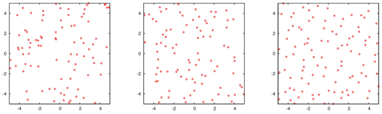
Fig. 1 Samples of the Poisson (α→0, left),α-Ginibre (α=0.5, center) and original Ginibre (α=1, right) point processes with the same intensity.[19]

that theα-Ginibre point process constitutes an intermediate class between the original Ginibre and homogeneous Pois- son point processes by the parameterα ∈ (0,1]. Figure 1 shows samples of the Poisson andα-Ginibre point processes with the same intensity. We can see that the configuration of the points becomes more regular as the value ofαbecomes larger.

Remark 1: As seen in (9), theα-Ginibre point process has the intensityπ⁻¹with respect to the Lebesgue measure; that is, forC∈ B(C),

EΦ(C)=

∫

C

ρ⁽¹⁾_α (z)να(dz)= µ(C) π .

However, we can consider the process with an arbitrary fixed intensity λ ∈ (0,∞) by scaling. The kernel and reference measure of the scaled α-Ginibre point process with inten- sityλ are respectively given byK_α,λ(z, w) =e^πλzw/α and να,λ(dz) = λe^−πλ|z|²^/αµ(dz). Or equivalently, the kernel KH_α,λ(z, w) = λe^−πλ(|z|²^+|w|²^)/(2α)e^πλzw/α with respect to the Lebesgue measureµdefines the same process.

We next see the nonzero eigenvalues and the corresponding eigenfunctions of the integral operator corresponding to the kernelK_α. Let

ϕα,i(z)= zⁱ⁻¹

√(i−1)!αⁱ, i∈N. (11) Then we can check that ϕα,i, i ∈ N, are the orthonormal eigenfunctions ofK_αcorresponding to the eigenvalueαsat- isfying

∫

Cϕα,i(z)ϕα,j(z)να(dz)=

{1 fori= j, 0 fori, j.

Thus, Mercer’s spectral expansion ([35]) holds such that K_α(z, w)=

∑∞ i=1

α ϕα,i(z)ϕα,i(w), z, w∈C.

Now, let D_r denote the disk on C centered at the origin with radiusr. Thenϕα,i,i∈N, in (11) are also orthogonal eigenfunctions (but not normal now) of the restrictionK_α,D_r

ofK_αonD_r corresponding to the eigenvalues κα,Dr,i =αP(i,r²/α)=αγ(i,r²/α)

Γ(i) , i∈N, (12) where P(x, y) = γ(x, y)/Γ(x) denotes the regularized lower Gamma function with the lower incomplete Gamma function γ(x, y) = ∫ _y

0 t^x⁻¹e⁻^tdt and the usual Gamma function Γ(x) = γ(x,∞). Let χi, i ∈ N, denote i.i.d.

Bernoulli random variables withP(χi =1) =αand letY_i, i ∈ N, denote mutually independent random variables with Y_i ∼Gam(i, α⁻¹), where{χi}i∈Nand{Y_i}i∈Nare also independent of each other. Then, sinceP(Y_i ≤r²)=P(i,r²/α), (5) and (12) imply

Φ_α(D_r)=^d ∑

i∈N

χi1_{Y_i_≤r2}.

This observation is closely related to the following proposition, which is a generalization of Kostlan’s result [36] for the original Ginibre point process (see also [26, Theorem 4.7.1]).

Proposition 2: LetX_i,i ∈ N, denote the points of theα- Ginibre point process. Then, the set{|X_i|²}i∈Nhas the same distribution as Yˇ = {Yˇ_i}i∈N, which is extracted from Y = {Y_i}i∈N such thatY_i,i ∈ N, are mutually independent with Y_i ∼Gam(i, α⁻¹)and eachY_i is added inYˇ with probability αand discarded with1−αindependently of others.

Indeed, theα-Ginibre point processΦ_αis obtained from the original Ginibre processΦ=Φ₁by retaining each point of Φwith probabilityα (removing it with1−α) independently, and then applying the homothety of ratio√αto the retained points in order to maintain the original intensity of the Ginibre process Φ ([28]). Proposition 2 is useful for analyzing the cellular network models described in the pre- ceding section since the path-loss function usually depends only on the distance from a BS. When we consider the scaled α-Ginibre point process with intensityλ ∈ (0,∞)as in Re- mark 1,Gam(i, α⁻¹)in the above proposition is replaced by Gam(i, πλ/α).

We can extend Proposition 2 to the process under the Palm distribution. Applying (6) to (7), the kernelK_α^oof the α-Ginibre point process under the reduced Palm distribution

(5)

given a point at the origin is

K_α^o(z, w)=e^zw/α−1, (13) with respect to the same reference measureναin (8). Thus, the first product density is given by

ρ^o(1)_α (z)να(dz)=K_α^o(z,z)να(dz)

= 1

π(1−e^−|z^|²^/α)µ(dz).

Note that theα-Ginibre point process is no longer stationary under the Palm distribution and the intensity function is increasing according to the distance from the origin. The following Proposition is obtained by applying the kernel (13) to Theorem 4.7.1 of[26].

Proposition 3: LetX_i^o,i ∈N, denote the points of theα- Ginibre point process under the reduced Palm distribution.

Then, the set{|X_iô|²}i∈Nhas the same distribution asYˇô = {Yˇ_iô}i∈N, which is extracted fromY ={Y_iô}i∈Nsuch thatY_iô, i∈N, are mutually independent withY_iô ∼Gam(i+1, α⁻¹) and eachY_iôis added inYˇôwith probabilityαand discarded with1−αindependently of others.

Note thatYˇ^o in Proposition 3 is obtained fromYˇ in Proposition 2 by removing the exponentially distributed random variableY₁ ∼Gam(1, α⁻¹)if it is retained with proba- bilityα(see[28]).

4. Coverage Analysis

In this section, we show some existing results on the coverage analysis of the cellular network models described in Sect. 2;

that is, we give the numerically computable forms of the coverage probability for the two examples in Sect. 2. Here, the coverage probability is defined as the tail probability P(SINR_o > θ),θ >0, of the SINR in (1), which represents the probability that the SINR for the typical user achieves a target thresholdθ.

4.1 Homogeneous Single-Antenna Network

We here derive a numerically computable form of the coverage probability for the homogeneous single-antenna network model in Example 1, where the BSs are deployed according to theα-Ginibre point process with intensityλ ∈(0,∞). The corresponding result for the model with Poisson deployed BSs is also derived. The proof for the Poisson deployed BS model mainly follows[11]while that for theα-Ginibre deployed BS model does[17],[19].

Theorem 1([11],[17],[19]): Consider the homogeneous single-antenna cellular network model in Example 1 with the path-loss functionℓ(r)=r^−2β,r >0, for β >1, where H_i ∼Exp(1),i ∈ N, (Rayleigh fading) andG_i,i ∈ N, are i.i.d. When the point processΦis the homogeneous Pois- son point process with intensity λ ∈ (0,∞), the coverage probability for the typical user is given by

P(SINR_o^(PPP)> θ)

=

∫ _∞

0

exp {−θ wo

p ( t

π λ )_β

−t(

1+τ(θ, β))}

dt, (14) where

τ(θ, β)= θ^1/β β

∫ _∞

1/θ

(1− LG(u⁻¹))

u^−1+1/βdu, (15) and LG denotes the Laplace transform ofG_i,i ∈ N. On the other hand, whenΦis theα-Ginibre point process with intensityλ,

P(SINR_o^(α-GPP)> θ)

=α

∫ _∞

0

exp

{−t−θ wo

p (αt

πλ )_β}

×M_α(t, θ, β)S_α(t, θ, β)dt, (16) where

M_α(t, θ, β)=

∏∞ i=0

[1−α+αJ_i(t, θ, β)]

, (17)

S_α(t, θ, β)=

∑∞ i=0

tⁱ i!

[1−α+αJ_i(t, θ, β)]₋₁

, (18)

with

J_i(t, θ, β)= 1 i!

∫ _∞

t

e^−uuⁱLG

(θ(t u

)_β)

du. (19) For the proof of (14)–(15) for the Poisson deployed BS model, we use the probability generating functional for point processes.

Definition 1: LetΦ = {X_i}i∈Ndenote a point process on R^dwith intensity measureΛ; that is,EΦ(C)=Λ(C)forC∈ B(R^d). For any measurable functionv: R^d → [0,1] such that ∫

R^d

(1−v(x))

Λ(dx) < ∞, the probability generating functional of the point processΦis defined as

GΦ(v)=^E[∏

i∈N

v(X_i) ].

Proposition 4(e.g.,[37, Sec. 9.4]): For the Poisson point processΦonR^d with intensity measureΛ, its probability generating functional is given as

G_Φ^(PPP)(v)=exp {−

∫

R^d

(1−v(x)) Λ(dx)

}. (20)

Note that, ifΦis stationary with intensityλ, thenΛ(dx) above is replaced byλdx.

Proof of Theorem 1:In the definition of the SINR in (1), each H_i is independent of Φ = {X_i}i∈N and {G_j}j∈N\{i}. Also, η(o) is determined by Φ = {X_i}i∈N. Thus, con- ditioning on Φ = {X_i}i∈N and {G_j}j∈N\{η(o)}, and using H_i ∼Exp(1),i∈N, we have

(6)

P(SINRo> θ)=P (

H_η_(o)> θ I_o(η(o))+wo

pℓ(|X_η(o)|) )

=E [

exp

{−θI_o(η(o))+wo

pℓ(|X_η_(o)|) }].

Furthermore, the definition of the interference (2) and the Laplace transform ofG_j,j∈N, lead to

P(SINR_o> θ)

=E [

exp

{− θ wo

pℓ(|X_η(o)|)

} ∏

j∈N\{η(o)}

LG

(θ ℓ(|X_j|) ℓ(|X_η_(o)|)

)],

(21) which is the starting point for the coverage analysis of both the Poisson and α-Ginibre deployed BS cellular network models.

We first show (14)–(15) for the Poisson deployed BS model. For the homogeneous Poisson point processΦ on R² with intensityλ, the distribution for the distance to the nearest point from the origin is given by

P(|X_η(o)| >r)=P(

Φ(D_r)=0)=e^−λπr², (22) where D_r denotes the disk centered at the origin with radiusr. Given |X_η_(o)| = r, other points of Φ also follow the Poisson point process onR²\D_r, and thus applying the probability generating functional (20), we obtain

E [∏

j∈N

LG

(θℓ(|X_j|) ℓ(r)

) X_j ∈R²\D_r, j∈N]

=exp {−λ

∫

|x|>r

[ 1− LG

(θℓ(|x|) ℓ(r)

)]

dx }

=exp {−2πλ

∫ _∞

r

[ 1− LG

(θℓ(s) ℓ(r)

)]

sds

}. (23)

Hence, applying (22), (23) andℓ(r) = r^−2β to (21) yields (14)–(15) after some manipulations.

On the other hand, for the α-Ginibre deployed BS model, we useY = {Y_i}i∈N in Proposition 2 such thatY_i, i ∈ N, are mutually independent and each Y_i is retained with probabilityαindependently of others. Thus, dividing the cases in each of which the point corresponding toY_i is retained and associated with the typical user, (21) with ℓ(r)=r^−2βreduces to

P(SINR^(α-GPP)_o > θ)

=α∑

i∈N

E [

exp {−θ wo

p Y_i^β }

× ∏

j∈N\{i}

{

1−α+αLG

(θ(Y_i Y_j

)_β) 1_{Y_j_≥Y_i_}

}].

Finally, applyingY_i∼Gam(i, πλ/α),i∈Nyields (16)–(19)

after some manipulations. □

Figure 2 shows the comparison result of the coverage probability with diﬀerent values ofα. Each plot indicates the coverage probability for a given value ofθin the case of

Fig. 2 Comparison of coverage probability in terms ofαin the single tier model (ℓ(r)=r⁻⁴, no noise).[19]

wo =0(noise-free) and β =2(i.e.,ℓ(r) =r⁻⁴). It seems that the coverage probability is increasing inα. However, a numerical result in[18]shows that the coverage probability is not always monotone inαasθ→ ∞.

4.2 Two-Tier Ginibre-Poisson Overlaid Network

In this subsection, we consider the case of K =2in Exam- ple 2, where the BSs of tier1are deployed according to the α-Ginibre point processΦ₁with intensityλ1while the BSs of tier2follow the homogeneous Poisson point processΦ₂ with intensityλ2. This represents the heterogeneous two-tier cellular network where the macro BSs are deployed rather systematically while the femto BSs are located in an oppor- tunistic manner. We assume that the two point processesΦ₁ andΦ₂ are independent of each other. In the coverage of users, the target thresholds can diﬀer for the two tiers; that is, the SINR should be larger thanθk when a user is served by a BS of tierkfork=1,2.

For the ease of understanding, we impose some extent of simplifying setting (see[23]for a general setting). First, we ignore the noise power and setwo =0, in this case, the SINR in (1) is called the signal-to-interference ratio (SIR).

Furthermore, we only consider the case where the number of users served at each BS is equal to the number of antennas;

that is, m_k = ψk for k = 1, 2. This case reduces to the single-input single-output (SISO) transmission whenm_k = ψk =1or the full form of space-division multiple access (full SDMA) transmission when m_k =ψk > 1. In this setting, H_i ∼Exp(1),i∈N, sinceδk =1for eachk∈ K, and they are mutually independent.

Theorem 2: Consider the two-tier multi-antenna cellular network model in Example 2 withK=2,ℓ1(r)=r^−2β¹and ℓ2(r)=r^−2β². Then, under the setting described above, the coverage probability for the typical user is given by

P(SIR^(MIMO)_o > θξη(o))

=α

∫ _∞

0

M_α(t, θ1, β1)S_α(t, θ1, β1) (24a)

(7)

×exp

{−t−C_α⁽¹^,²⁾(t)(

1+τ1,2(θ1, β2)}

dt (24b) +

∫ _∞

0

M_α^(2,1)(t, θ2, β1, β2) (24c)

×exp{

−t(

1+τ(θ2, β2))}

dt (24d)

whereM_α(t, θ, β)andS_α(t, θ, β)are the same as in (17) and (18) respectively withLG(s)=LG,1(s)=(1+s)^−ψ¹ inJ_i in (19). Moreover,

C_α^(1,2)(t)=πλ2

(b₂p₂ b₁p₁

)_1/β2( αt πλ1

)_β1/β2

, τ1,2(θ, β)=θ^1/β

β

∫ _∞

1/θ

[

1−( u u+b₁/b₂

)_ψ2]

u^−1+1/βdu, and

M_α^(2,1)(t, θ, β1, β2)=

∏∞ i=0

[1−α+αJ_α,^(2,1)_i (t, θ, β1, β2)] , where

J_α,i^(2,1)(t, θ, β1, β2)

= 1 i!

∫ _∞

C_α⁽²^,¹⁾(t)

e^−uuⁱ [

1+θp₁ p₂

(t/πλ2)^β² (αu/πλ1)^β¹

]−ψ1

du, with

C_α^(2,1)(t)= πλ1

α (b₁p₁

b₂p₂

)1/β1( t πλ2

)β2/β1

.

τ(θ, β) is also the same as in (15) with LG(u⁻¹) = LG,2(u⁻¹)=[

u/(u+1)]_ψ₂ .

The proof is placed in the appendix and we here make a short remark on Theorem 2. The formula of the coverage probability in the theorem consists of two parts (24a)–(24b) and (24c)–(24d). The first part corresponds to that the typical user is served by a BS of tier1, so that the term in (24a) is given as the same form as in (16). The term in (24b) corresponds to the cumulative interference from all the BSs of tier 2, which can be seen similar to the second term in the exponential in (14). The second part (24c)–(24d) corresponds to that the typical user is served by a BS of tier2, so that the term in (24d) has the same form as the second term in the exponential in (14). The term in (24c) corresponds to the cumulative interference from all the BSs of tier1, so thatM_α⁽²^,¹⁾has a similar form toM_αin (17) (the term corresponding toS_αdoes not appear in this case).

5. Conclusion

In this tutorial, we have introduced theα-Ginibre point process as the model of BS deployments in cellular networks.

First, we have reviewed the definition and some useful properties of this process, and then we have seen the two existing results on the coverage analysis of cellular network models, where the BSs are deployed according to theα-Ginibre point

processes. The authors now hope that the readers will use the (α-)Ginibre point process and challenge themselves to various problems arising in future cellular networks.

Finally, when we use the Ginibre and other determinantal point processes as the models of BS deployments, we might face to a computation problem. Although the obtained formulas are indeed numerically computable, as seen in (16)–(19) and (24a)–(24d), they include infinite sums and infinite products, which may lead to the time-consuming computation. One direction to avoid this problem could be some kinds of asymptotics and/or approximation (see, e.g., [18],[21],[38]–[40]for this direction).

Acknowledgments

The first author’s work was supported by the Japan Society for the Promotion of Science (JSPS) Grant-in-Aid for Sci- entific Research (C) 16K00030. The second author’s work was supported by JSPS Grant-in-Aid for Scientific Research (B) 26287019.

References

[1] J. Andrews, R. Ganti, M. Haenggi, N. Jindal, and S. Weber, “A primer on spatial modeling and analysis in wireless networks,” IEEE Commun. Mag., vol.48, no.11, pp.156–163, 2010.

[2] M. Haenggi, J.G. Andrews, F. Baccelli, O. Dousse, and M.

Franceschetti, “Stochastic geometry and random graphs for the analysis and design of wireless networks,” IEEE J. Sel. Areas. Commun., vol.27, no.7, pp.1029–1046, 2009.

[3] H. ElSawy, E. Hossain, and M. Haenggi, “Stochastic geometry for modeling, analysis, and design of multi-tier and cognitive cellular wireless networks: A survey,” IEEE Commun. Surv. Tutorials, vol.15, no.3, pp.996–1019, 2013.

[4] H. ElSawy, A. Sultan-Salem, M.S. Alouini, and M.Z. Win, “Model- ing and analysis of cellular networks using stochastic geometry: A tutorial,” arXiv: 1604.03689 [cs.IT], 2016.

[5] F. Baccelli and B. Błaszczyszyn, “Stochastic geometry and wireless networks: Volume I theory,” Foundations and Trends®in Network- ing, vol.3, no.3-4, pp.249–449, 2009.

[6] F. Baccelli and B. Błaszczyszyn, “Stochastic geometry and wireless networks: Volume II applications,” Foundations and Trends®in Networking, vol.4, no.1-2, pp.1–312, 2009.

[7] M. Haenggi, Stochastic Geometry for Wireless Networks, Cambridge Univ. Press, 2013.

[8] S. Mukherjee, Analytical Modeling of Heterogeneous Cellular Net- works: Geometry, Coverage, and Capacity, Cambridge Univ. Press, 2014.

[9] H. ElSawy and E. Hossain, “Two-tier HetNets with cognitive fem- tocells: Downlink performance modeling and analysis in a multi- channel environment,” IEEE Trans. Mobile Comput., vol.13, no.3, pp.649–663, 2014.

[10] M. Wildemeersch, T.Q.S. Quek, M. Kountouris, A. Rabbachin, and C.H. Slump, “Successive interference cancellation in heterogeneous networks,” IEEE Trans. Commun., vol.62, no.12, pp.4440–4453, 2014.

[11] J.G. Andrews, F. Baccelli, and R.K. Ganti, “A tractable approach to coverage and rate in cellular networks,” IEEE Trans. Commun., vol.59, no.11, pp.3122–3134, 2011.

[12] H.S. Dhillon, R.K. Ganti, F. Baccelli, and J.G. Andrews, “Modeling and analysis ofK-tier downlink heterogeneous cellular networks,”

IEEE J. Sel. Areas. Commun., vol.30, no.3, pp.550–560, 2012.

[13] H.-S. Jo, Y.J. Sang, P. Xia, and J.G. Andrews, “Heterogeneous cellu-

(8)

lar networks with flexible cell association: A comprehensive downlink SINR analysis,” IEEE Trans. Wireless Commun., vol.11, no.10, pp.3484–3495, 2012.

[14] S. Mukherjee, “Distribution of downlink SINR in heterogeneous cellular networks,” IEEE J. Sel. Areas. Commun., vol.30, no.3, pp.575–

585, 2012.

[15] M.D. Renzo, A. Guidotti, and G.E. Corazza, “Average rate of downlink heterogeneous cellular networks over generalized fading channels: A stochastic geometry approach,” IEEE Trans. Commun., vol.61, no.7, pp.3050–3071, 2013.

[16] A. Guo and M. Haenggi, “Spatial stochastic models and metrics for the structure of base stations in cellular networks,” IEEE Trans.

Wireless Commun., vol.12, no.11, pp.5800–5812, 2013.

[17] N. Miyoshi and T. Shirai, “A cellular network model with Ginibre configured base stations,” Adv. Appl. Probab., vol.46, no.3, pp.832–

845, 2014.

[18] N. Miyoshi and T. Shirai, “Cellular networks withα-Ginibre config- urated base stations,” The Impact of Applications on Mathematics, Mathematics for Industry, vol.1, pp.211–226, Springer Japan, Tokyo, 2014.

[19] I. Nakata and N. Miyoshi, “Spatial stochastic models for analysis of heterogeneous cellular networks with repulsively deployed base stations,” Perform. Evaluation., vol.78, pp.7–17, 2014.

[20] T. Kobayashi and N. Miyoshi, “Uplink cellular network models with Ginibre deployed base stations,” 2014 26th International Teletraﬃc Congress (ITC), pp.1–7, 2014.

[21] H. Nagamatsu, N. Miyoshi, and T. Shirai, “Padé approximation for coverage probability in cellular networks,” 2014 12th International Symposium on Modeling and Optimization in Mobile, Ad Hoc, and Wireless Networks (WiOpt), pp.693–700, 2014.

[22] N. Miyoshi and T. Shirai, “Downlink coverage probability in a cellular network with Ginibre deployed base stations and Nakagami-m fading channels,” 2015 13th International Symposium on Model- ing and Optimization in Mobile, Ad Hoc, and Wireless Networks (WiOpt), pp.483–489, 2015.

[23] T. Kobayashi and N. Miyoshi, “Downlink coverage probability in Ginibre-Poisson overlaid MIMO cellular networks,” 2016 14th In- ternational Symposium on Modeling and Optimization in Mobile, Ad Hoc, and Wireless Networks (WiOpt), pp.1–8, 2016.

[24] A. Soshnikov, “Determinantal random point fields,” Russ. Math.

Surv., vol.55, no.5, pp.923–975, 2000.

[25] T. Shirai and Y. Takahashi, “Random point fields associated with certain Fredholm determinants I: Fermion, Poisson and Boson point processes,” J. Funct. Anal., vol.205, no.2, pp.414–463, 2003.

[26] J.B. Hough, M. Krishnapur, Y. Peres, and B. Virág, “Determinantal point processes,” Zeros of Gaussian Analytic Functions and Determi- nantal Point Processes, University Lecture Series, vol.51, pp.47–81, American Mathematical Society, Providence, Rhode Island, 2009.

[27] F. Lavancier, J. Møller, and E. Rubak, “Determinantal point process models and statistical inference,” J. R. Stat. Soc. B, vol.77, no.4, pp.853–877, 2015.

[28] A. Goldman, “The Palm measure and the Voronoi tessellation for the Ginibre process,” Ann. Appl. Probab., vol.20, no.1, pp.90–128, 2010.

[29] N. Deng, W. Zhou, and M. Haenggi, “The Ginibre point process as a model for wireless networks with repulsion,” IEEE Trans. Wireless Commun., vol.14, no.1, pp.107–121, 2015.

[30] J.S. Gomez, A. Vasseur, A. Vergne, P. Martins, L. Decreusefond, and W. Chen, “A case study on regularity in cellular network deployment,” IEEE Wireless Commun. Lett., vol.4, no.4, pp.421–424, 2015.

[31] Y. Li, F. Baccelli, H.S. Dhillon, and J.G. Andrews, “Statistical modeling and probabilistic analysis of cellular networks with determinantal point processes,” IEEE Trans. Commun., vol.63, no.9, pp.3405–

3422, 2015.

[32] H. Huang, C.B. Papadias, and S. Venkatesan, MIMO Communica- tion for Cellular Networks, Springer, 2012.

[33] H.S. Dhillon, M. Kountouris, and J.G. Andrews, “Downlink MIMO HetNets: Modeling, ordering results and performance analysis,”

IEEE Trans. Wireless Commun., vol.12, no.10, pp.5208–5222, 2013.

[34] A.K. Gupta, H.S. Dhillon, S. Vishwanath, and J.G. Andrews, “Down- link coverage probability in MIMO HetNets with flexible cell selec- tion,” 2014 IEEE Global Communications Conference, pp.1534–

1539, 2014.

[35] J. Mercer, “Functions of positive and negative type, and their connec- tion with the theory of integral equations,” Philosophical Transac- tions of the Royal Society A: Mathematical, Physical and Engineering Sciences, vol.209, no.441-458, pp.415–446, 1909.

[36] E. Kostlan, “On the spectra of Gaussian matrices,” Linear Algebra Appl., vol.162-164, pp.385–388, 1992.

[37] D.J. Daley and D. Vere-Jones, An Introduction to the Theory of Point Processes, Volume II: General Theory and Structure, Second ed., Springer, 2008.

[38] R.K. Ganti and M. Haenggi, “Asymptotics and approximation of the SIR distribution in general cellular networks,” IEEE Trans. Wireless Commun., vol.15, no.3, pp.2130–2143, 2016.

[39] H. Wei, N. Deng, W. Zhou, and M. Haenggi, “Approximate SIR analysis in general heterogeneous cellular networks,” IEEE Trans.

Commun., vol.64, no.3, pp.1259–1273, 2016.

[40] N. Miyoshi and T. Shirai, “A suﬃcient condition for tail asymptotics of SIR distribution in downlink cellular networks,” 2016 14th Inter- national Symposium on Modeling and Optimization in Mobile, Ad Hoc, and Wireless Networks (WiOpt), pp.1–7, 2016.

Appendix: Proof of Theorem 2

We divide the coverage probability into two cases according to the tier of the BS associated with the typical user;

P(

SIR^(MIMO)_o > θξ_η(o)

)=P(

SIR^(MIMO)_o > θ1, ξη(o)=1) +^P(

SIR^(MIMO)_o > θ2, ξη(o)=2) , (A·1) and consider the two terms separately.

(1) Case ofξη(o)=1:

LetN1 andN2 denote the random partition ofNsuch that Nk ={i ∈N:ξi=k}fork=1,2. Then, the interference (2) fori∈N1is written as

I_o(i)= ∑

j∈N1\{i}

p₁G_jℓ1(|X_j|)+∑

j∈N2

p₂G_jℓ2(|X_j|). Applying this to the first term on the right-hand side of (A·1) yields

P(

SIR_o^(MIMO)> θ1, ξη(o)=1)

=^E [

exp {−θ1

I_o(η(o)) p₁ℓ1(|X_η(o)|)

}

1_{ξ_η_(o)₌₁_} ]

=E

[ ∏

j∈N1\{η(o)}

LG,1

( θ1

(|X_η(o)|

|X_j| )2β1)

× ∏

j∈N2

LG,2

( θ1

p₂ p₁

|X_η(o)|^2β¹

|X_j|^2β² )

1_{ξ_η_(o)₌1}

]

, (A·2)

whereℓ1(r) =r^−2β¹ andℓ2(r)=r^−2β² are also used. Note here that {η(o) =i}withi ∈ N1 implies{|X_j| ≥ |X_i|}for