derived the maximum likelihood estimator for the population mean vec- tor and the population covariance matrix. Then Tsukada[8] derived the unbiased estimator for the covariance matrix.

−31−

Shin-ichi TSUKADA

Estimation of covariance matrix for Stein’s loss on a two-step monotone incomplete sample

Abstract

For a two-step monotone incomplete sample, it is known that Anderson[1]

derived the maximum likelihood estimator for the population mean vec- tor and the population covariance matrix. Then Tsukada[8] derived the unbiased estimator for the covariance matrix.

On the other hand, Richards and Yamada[6] estimated the mean vector based on the loss function. In this article, we deal with the inference for the covariance matrix based on Stein’s loss function. The estimator, which has the minimum risk, is proposed, and we compare the risks of the maximum likelihood estimator with the unbiased estimator, and with the proposed estimator, respectively.

Keywords. Stein’s loss, Risk, Covariance matrix, Monotone incomplete sample

1 Introduction

We consider a monotone incomplete data, which was drawn from a multivari- ate normal population consisting of mutually independent observations of the following form;

X 1

Y 1

,

X 2

Y 2

, . . . ,

X n

Y n

,

X n+1

∗

, . . . , X N

∗

, (1)

where each X i ∈ R ^p and each Y i ∈ R ^q ; (X i , Y i ) ⁰ , i = 1, . . . , n are observations from N p+q (µ, Σ), and the incomplete data X i , i = n+1, . . . , N, are observations of the first p elements of the same population.

To ensure that all means and variances are finite and that all integrals sub- sequently encountered are absolutely convergent, we also assume that n > p + 2 and N > n ≥ p + q (Chang and Richards[3]). As explained by Yamada, et al.[9], we also assume that data are missing completely at random to derive the maximum likelihood estimators ˆ µ and ˆ Σ.

Anderson[1] and Anderson and Olkin[2] derived the maximum likelihood es- timator (MLE) for µ and Σ, while Kanda and Fujikoshi[5] investigated some of

∗

School of Education, Meisei University. 2-1-1 Hodokubo Hino City Tokyo 191-8506, JAPAN. E-mail:[email protected].

1

−32−

their properties. Chang and Richards[3],[4] derived a stochastic representation for the exact distribution of the MLE ˆ µ and ˆ Σ for a two-step monotone incom- plete sample. They obtained an ellipsoidal confidence region for µ, and con- sidered hypothesis testing for the covariance matrix. Richards and Yamada[6]

studied the Stein phenomenon for a two-step monotone sample. They derived an improved estimator for µ. Recently, Tsukada[8] derived an unbiased estimator (UBE) for Σ and investigated its properties.

In this paper, we consider the inference for the covariance matrix Σ us- ing Stein’s loss function on a two-step monotone incomplete sample. We have obtained a new estimator and have discussed its properties in Section 2. In Sec- tion 3, we investigate the accuracy of the new estimator by performing numerical simulations.

2 Estimation of covariance matrix for Stein’s loss

Let the missing ratio be τ = (N − n)/N . We decompose µ and Σ as follows;

µ = µ ₁

µ ₂

, Σ =

Σ ₁₁ Σ ₁₂ Σ ₂₁ Σ ₂₂

,

where µ ₁ and µ ₂ are a p-element vector and q-element vector, respectively; Σ ₁₁ , Σ ₁₂ = Σ ⁰ ₂₁ , and Σ ₂₂ are of orders p × p, p × q, and q × q, respectively. We also define the Schurz complement Σ _22·1 = Σ ₂₂ − Σ ₂₁ Σ ⁻¹ ₁₁ Σ ₁₂ .

Define the sample mean vectors X ¯ 1 = 1

n X n i=1

X i , X ¯ 2 = 1 N − n

X N i=n+1

X i , Y ¯ = 1

n X n i=1

Y _i , X ¯ = 1 N

X N i=1

X _i ,

and the corresponding matrices of the sums of squares and products A 11,n =

X n i=1

X i − X ¯ 1

X i − X ¯ 1

⁰

, A 12 = A ⁰ ₂₁ = X n i=1

X i − X ¯ 1

Y i − Y ¯ ⁰ , A 22 =

X n i=1

Y i − Y ¯

Y i − Y ¯ ⁰

, A 11,N = X N i=1

X i − X ¯

X i − X ¯ ⁰ . The MLE is represented as follows:

ˆ

µ ₁ = ¯ X , µ ˆ ₂ = ¯ Y − (1 − τ)A ₂₁ A ⁻¹ _11,n X ¯ ₁ − X ¯ ₂

, (2)

−33−

Σ ˆ 11 = 1

N A 11,N , Σ ˆ 12 = 1

N A 11,N A ⁻¹ _11,n A 12 , (3)

Σ ˆ ₂₂ = 1

n A _22·1,n + 1

N A ₂₁ A ⁻¹ _11,n A _11,N A ⁻¹ _11,n A ₁₂ . As shown by Kanda and Fujikoshi[5], the expectation of ˆ Σ is

E h Σ ˆ i

= N − 1 N Σ + b ₀

N

O O O Σ _22·1

, where

b ₀ = − (N − n) {n − (p + 1)(p + 2)}

n(n − p − 2) . The MLE is biased. Tsukada[8] proposes the UBE ˜ Σ as follows:

Σ ˜ 11 = N N − 1

Σ ˆ 11 , Σ ˜ 12 = N N − 1

Σ ˆ 12 , Σ ˜ 22 = N N − 1

Σ ˆ 22 − c 0 Σ ˆ 22·1 , (4) where

c 0 = (N − n)(p + 1)(p + 2) − n(N − n) (N − 1)(n − p − 2)(n − p − 1) ,

and shows that the risk of the UBE is smaller than the risk of MLE for Stein’s loss. By expanding the MLE and the UBE, the asymptotic distribution of these estimators was derived.

Let Λ ₁₁ and Λ ₂₂ be p×p and q×q positive definite matrices, respectively. Let Λ ₂₁ be a q × p matrix and let ν ₁ and ν ₂ be p × 1 and q × 1 vectors, respectively.

We define Λ =

Λ ₁₁ O O Λ ₂₂

, C =

I _p O Λ ₂₁ I _q

, ν = ν ₁

ν ₂

, (5)

and consider the set of affine transformations of the data in (1) to be of the

form

X ^∗ _i Y ^∗ _i

= ΛC X _i

Y _i

+ ν, i = 1, . . . , n, X ^∗ _j = Λ ₁₁ X _j + ν ₁ , j = n + 1, . . . , N.

(6)

Romer and Richards[7] also considered the transformation in (6), and noted that as Λ ₁₁ , Λ ₂₁ , Λ ₂₂ , and ν vary over their respective parameter spaces. The set of all transformations in (6) forms a group; in particular, each such transformation is invertible.

We consider a class of estimators, which is of the form

Σ ¨ ≡ d 1 Σ ˆ + d 2

O O O Σ ˆ 22·1

d 1 , d 2 ∈ R

. (7)

−34−

This class is invariant for the transformation in (6), and includes the MLE and UBE. We derive the estimator, which minimizes the risk for Stein’s loss function

L(A, Σ) = tr Σ ⁻¹ A

− log |A|

|Σ| − (p + q), (8) where A is an estimator of Σ. We calculate the risk of this class of estimators as follows:

R Σ, ¨ Σ

= R

d 1 Σ ˆ + d 2

O O O Σ ˆ _22·1

, Σ

= d 1 E h

trΣ ⁻¹ Σ ˆ i + d 2 E

trΣ ⁻¹

O O O Σ ˆ _22·1

−E

log

Σ ¨ 11 Σ ¨ 12

Σ ¨ ₂₁ Σ ¨ ₂₂

− log |Σ|

− (p + q). (9) Since

E h

trΣ ⁻¹ Σ ˆ i

= N − 1

N (p + q) + b ₀ N q, E

trΣ ⁻¹

O O O Σ ˆ _22·1

= n − p − 1 n q, E

log

Σ ¨ ₁₁ Σ ¨ ₁₂ Σ ¨ 21 Σ ¨ 22

− log |Σ|

= E



log Σ ¨ 11

|Σ ₁₁ | + log Σ ¨ 22·1

|Σ _22·1 |





= p log |d 1 | + M 11 + q log |d 1 + d 2 | + M 22·1 , where

M 11 = E



log Σ ˆ ₁₁

|Σ 11 |



 = −p log N

2

+ X p i=1

Γ ⁰ [(N − i)/2]

Γ [(N − i)/2] ,

M _22·1 = E



log Σ ˆ _22·1

|Σ _22·1 |



 = −q log n 2

+ X q i=1

Γ ⁰ [(n − p − i)/2]

Γ [(n − p − i)/2] , the risk is

R( ¨ Σ, Σ) = d 1

N − 1

N (p + q) + b ₀ N q

+ d 2 · n − p − 1

n q

−p log |d ₁ | − M ₁₁ − q log |d ₁ + d ₂ | − M _22·1 − (p + q). (10) By differentiating the risk and assuming zero, we consider d ₁ and d ₂ in order to

4

−35−

minimize the risk as follows:

d ₁ = N (n − p − 2)

N (n − p + q − 2) − n − (p + 2)(q − 1)

= (1 − τ )N ² − N (p + 2)

(1 − τ )N ² − N(p − q + 3 − τ ) − (p + 2)(q − 1) , (11) d 2 = N {(p + 1)(p + 2) − n(p + q + 1)} + n(p + 2)(q − 1) + n ²

N (n − p − 1)(n − p + q − 2) − (n − p − 1) {n + (p + 2)(q − 1)}

= N ² (1 − τ )(p + q + τ) − N(p + 2)(p + q + τ − τ q)

F (N ) , (12)

where

F (N) = N ³ (1 − τ) ² + N ² (2p − q + 4 − τ )

+N

p ² + p(5 − 2q + τ q − 2τ) − 3q + 2τ q − 3τ + 5 +(p + 1)(p + 2)(q − 1).

Therefore, we obtain the following theorem.

Theorem 2.1. We again denote the estimator as Σ ¨ and call the minimum risk estimator by this estimator, when d 1 is (11) and d 2 is (12). Since the minimum of the risk is

R( ¨ Σ, Σ) = −p log

N(n − p − 2)

N(n − p + q − 2) − n − (p + 2)(q − 1)

−q log

n n − p − 1

− M ₁₁ − M _22·1 ,

the difference between the risk of the MLE and that of the minimum risk esti- mator is

R( ˆ Σ, Σ) − R( ¨ Σ, Σ)

= − p + q N + b ₀

N q +p log

N (n − p − 2)

N (n − p + q − 2) − n − (p + 2)(q − 1) + q log

n n − p − 1

. Proof. Because the risk of the MLE is

R Σ, ˆ Σ

= − p + q N + b ₀

N q − M 11 − M 22·1 , (13) from Tsukada[8], the difference between the risk of the MLE and that of the minimum risk estimator is obtained.

Also, the expectation of this estimator is as follows:

5

−36−

Theorem 2.2. The expectation of the risk minimum estimator is E h

Σ ¨ i

= a 1 Σ + a 2

O O O Σ _22·1

, (14)

where

a 1 = (N − 1)(n − p − 2)

N(n − p + q − 2) − n − (p + 2)(q − 1) ,

a ₂ = n ² − nN (p + q + 1) + N(p + 1)(p + 2) + n(p + 2)(q − 1) n ² (N − 1) − N(p − q + 2) − n(p + 2)(q − 1) . Proof. We can obtain this result using the following expectations:

E h Σ ˆ i

= N − 1 N Σ + b 0

N

O O O Σ 22·1

, E h

Σ ˆ 22·1

i

=

N − 1

N − p

N · N − p − 2

n − p − 2 − B ₀ N(n − p − 2)

Σ 22

+ b ₀

N + B ₀

N(n − p − 2)

Σ _22·1 , where

B 0 = n ² + n(N − n − 2p − 3) − (p + 1)(2N − 2n − p − 2).

The asymptotic distribution of this estimator is derived in a manner that is similar to the case of the MLE and the UBE.

Theorem 2.3. The estimator

√ N

vec

Σ ¨ ₁₁ − Σ ₁₁ , vec

Σ ¨ ₁₂ − Σ ₁₂ , vec

Σ ¨ ₂₂ − Σ ₂₂ ⁰

is asymptotically distributed as a normal distribution with mean vector 0 and a covariance matrix

Θ =



 Θ ₁₁ Θ ₁₂ Θ ₁₃ Θ ⁰ ₁₂ Θ ₂₂ Θ ₂₃ Θ ⁰ ₁₃ Θ ⁰ ₂₃ Θ ₃₃



 , (15) where K _ij is a commutation matrix and

Θ ₁₁ = (I _p

+ K _pp ) (Σ ₁₁ ⊗ Σ ₁₁ ) , Θ ₁₂ = (I _p

+ K _pp ) (Σ ₁₂ ⊗ Σ ₁₁ ) , Θ ₁₃ = (I _p

+ K _pp ) (Σ ₁₂ ⊗ Σ ₁₂ ) ,

Θ ₂₂ = 1

1 − τ (Σ ₂₂ ⊗ Σ ₁₁ ) − τ

1 − τ Σ ₂₁ Σ ⁻¹ ₁₁ Σ ₁₂ ⊗ Σ ₁₁

+ K _qp (Σ ₁₂ ⊗ Σ ₂₁ ) , Θ 23 = 1

1 − τ (Σ 22 ⊗ Σ 12 ) (I _q

+ K qq )

− τ

1 − τ Σ 21 Σ ⁻¹ ₁₁ Σ 12 ⊗ Σ 12

(I _q

+ K qq ),

Θ ₃₃ = 1

1 − τ (I _q

+ K _qq ) (Σ ₂₂ ⊗ Σ ₂₂ )

− τ

1 − τ (I _q

+ K _qq ) Σ ₂₁ Σ ⁻¹ ₁₁ Σ ₁₂ ⊗ Σ ₂₁ Σ ⁻¹ ₁₁ Σ ₁₂

.

−37−

Proof. When the sample size N increases, the coefficient d ₁ and d ₂ including Σ ¨ converge to 1 and 0, respectively. Furthermore, according to Tsukada[8], the asymptotic distribution of the estimator ¨ Σ is the same as that of the MLE.

The differences between the risks in Theorem 2.1, the expectation, and the convergence to the asymptotic distribution are evaluated in the next Section.

3 Numerical simulation

We perform numerical simulations to verify the expectation of the minimum risk estimator and the convergence to the asymptotic distribution of the estimator obtained in Section 2. Also, the risks were evaluated by numerical calculations.

3.1 Asymptotic distribution

We define the population distribution as follows. Write by

P =



 

 

 

 



1 ρ ρ ² ρ ³ ρ ⁴ ρ ⁵ ρ ⁶ ρ 1 ρ ρ ² ρ ³ ρ ⁴ ρ ⁵ ρ ² ρ 1 ρ ρ ² ρ ³ ρ ⁴ ρ ³ ρ ² ρ 1 ρ ρ ² ρ ³ ρ ⁴ ρ ³ ρ ² ρ 1 ρ ρ ² ρ ⁵ ρ ⁴ ρ ³ ρ ² ρ 1 ρ ρ ⁶ ρ ⁵ ρ ⁴ ρ ³ ρ ² ρ 1



 

 

 

 



and Λ = diag(σ ⁶ , σ ⁵ , . . . , σ ² , σ, 1).

We assume that the population distribution is the 7-variate normal distribution with mean vector 0 and the covariance matrix Σ = ΛP Λ. Let p = 4 and q = 3.

We set ρ = 0.15 and σ = √

2. The total sample sizes N are 500 and 1000. The missing rates τ are 0.2, 0.4, 0.6, and 0.8. The number of simulations performed was ten thousand.

Let v =

√ N

vec

Σ ¨ ₁₁ − Σ ₁₁ , vec

Σ ¨ ₁₂ − Σ ₁₂ , vec

Σ ¨ ₂₂ − Σ ₂₂ ⁰ . To investigate the convergence to the asymptotic distribution, we simulated the lower probability of v ⁰ Θ ⁻¹ v for the percentile of the chi-squared distribution with (p + q)(p + q + 1)/2 = 28 degrees of freedom. Table 1 denotes the result in the case of N = 500, and Table 2 denotes the result in the case of N = 1000.

The convergence in the case of N = 1000 is better than that in the case of

N = 500. As the missing rate τ increases, the convergence to the asymptotic

distribution worsens, but we find that the distribution of the estimator almost

converged to the asymptotic distribution for a range of more than 90%. Because

most of the lower probability for N = 500 and N = 1000 converge when τ =

20%, it is believed that we can use the asymptotic distribution in the case of

τ ≤ 20% and N ≥ 500.

−38−

Table 1: The lower probability for N = 500.

τ 1% 5% 10% 50% 90% 95% 99%

20% .0095 .0483 .0976 .5076 .9066 .9541 .9912 40% .0089 .0458 .0950 .5029 .9076 .9548 .9913 60% .0079 .0422 .0887 .4980 .9067 .9553 .9916 80% .0048 .0291 .0666 .4560 .8979 .9505 .9903

Table 2: The lower probability for N = 1000.

τ 1% 5% 10% 50% 90% 95% 99%

20% .0094 .0484 .0984 .5053 .9045 .9530 .9905 40% .0095 .0482 .0978 .5027 .9041 .9520 .9904 60% .0090 .0461 .0941 .4941 .9019 .9516 .9905 80% .0068 .0387 .0827 .4767 .8996 .9505 .9899

3.2 Expectation of the minimum risk estimator

We assume that the population distribution is the same as mentioned in the above subsection and the number of simulations is ten thousand, and we inves- tigated the expectation of the minimum risk estimator. The symbol S denotes the expectation of the minimum risk estimator obtained by simulation. To in- vestigate the accuracy of equation (14), we simulated as follows. We estimate the expectation as

S = (s ij ) = 1 N s

N

X

k=1

Σ ¨ k ,

where N _s is the number of simulations and ¨ Σ _k is the minimum risk estimator in each simulation, and we calculate the error

E =

p+q

X

i=1 p+q

X

j=i

(s

− E[¨ σ

])

= X

i=1

X

j=i

(s

− E[¨ σ

])

+ X

i=1 p+q

X

j=p+1

(s

− E[¨ σ

])

+

p+q

X

i=p+1 p+q

X

j=i

(s

− E[¨ σ

])

≡ E

+ E

+ E

.

In each Table, the notation x ^y indicates the value x × 10 ^y .

Because each error is almost the same when N = 200 and N = 500, and the total error is considered to be a range of simulation errors: thus, the expectation (14) appears to be correct.

8

−39−

Table 3: Error between the expectation obtained by the simulation and expec- tation in (14)

N = 200 N = 500

τ E ₁₁ E ₁₂ E ₂₂ E E ₁₁ E ₁₂ E ₂₂ E

20% 7.342 ⁻⁴ 9.571 ⁻⁵ 8.516 ⁻⁵ 9.150 ⁻⁴ 1.618 ⁻⁴ 1.973 ⁻⁵ 9.370 ⁻⁶ 1.909 ⁻⁴ 40% 1.598 ⁻⁴ 2.810 ⁻⁵ 3.463 ⁻⁴ 5.342 ⁻⁴ 2.787 ⁻⁴ 2.761 ⁻⁵ 5.856 ⁻⁵ 3.649 ⁻⁴ 60% 6.616 ⁻⁴ 5.607 ⁻⁵ 1.541 ⁻³ 2.259 ⁻³ 2.094 ⁻⁴ 3.500 ⁻⁵ 2.378 ⁻⁴ 4.821 ⁻⁴ 80% 4.047 ⁻⁴ 4.105 ⁻⁵ 7.917 ⁻³ 8.363 ⁻³ 1.198 ⁻⁴ 6.271 ⁻⁵ 1.221 ⁻³ 1.403 ⁻³

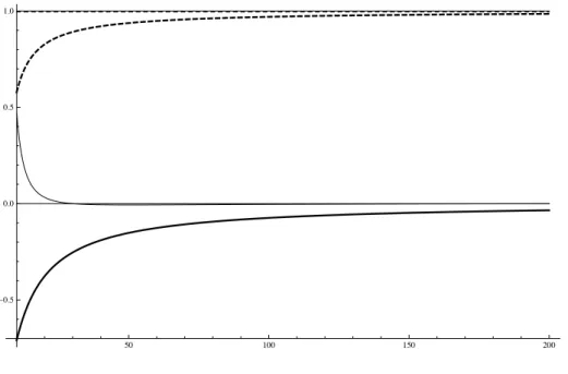
In the given scenario, we calculated the coefficients for Σ and Σ 22·1 in the case of N = 200 (Figure 1). The thin dashed line denotes the coefficient of the MLE and the dashed line denotes that of the minimum risk estimator. Similarly, the thin line denotes the coefficient for Σ 22·1 of the MLE and the line does that of the minimum risk estimator. One sees that the coefficient for Σ converges to 1 and the coefficient for Σ 22·1 converges to 0 as the missing rate τ decreases.

By considering the speed of convergence of each coefficient, we have that the MLE is better than the minimum risk estimator from a biased perspective.

50 100 150 200

-0.5 0.0 0.5 1.0

Figure 1: Coefficients in the case of N = 200

9

−40−

0.1 0.2 0.3 0.4

0.0005 0.0010 0.0015 0.0020 0.0025 0.0030 0.0035

0.5 0.6 0.7 0.8

0.005 0.010 0.015 0.020 0.025 0.030 0.035

Figure 2: Difference in Risk for N = 200

3.3 Risk of estimators

We investigated the difference in the risk of the MLE and the UBE, and the difference in the risk of the MLE and that of the minimum risk estimator.

Because the differences in the risks depend on the sample sizes N and n, and the dimensions p and q, we adopted the above setting as these parameters. In each figure, the dashed line denotes the difference in the risk of the MLE, and the thin line denotes the difference in the risk of the MLE and that of the minimum risk estimator.

The risks decrease when the sample size N increases. However, there are similar tendencies in both cases (N = 200 and N = 500). As the missing rate τ increases, the risks also increase. We have that the risk of the minimum risk estimator was the smallest, and the risk of the unbiased estimator was smaller than the risk of the MLE.

0.1 0.2 0.3 0.4

0.0001 0.0002 0.0003 0.0004 0.0005

0.5 0.6 0.7 0.8

0.001 0.002 0.003 0.004 0.005

Figure 3: Difference in Risk for N = 500

1

−41−

4 Conclusions

We derived an estimator, which has the minimum risk for Stein’s loss on a class of estimators, and investigated their properties. We obtained that its asymptotic distribution is the same as that of the MLE, but the estimator is biased. We are preparing to submit the result for the quadratic loss, and in future, we hope to study cases for other loss functions.

References

[1] T. W. Anderson, Maximum likelihood estimators for a multivariate normal distribution when some observations are missing, J. Am. Stat. Assoc., 52 (1957), 200–203.

[2] T. W. Anderson and L. Olkin, Maximum likelihood estimation of the pa- rameters of a multivariate normal distribution, Linear Algebra Appl., 70 (1985), 147–171.

[3] W. -Y. Chang and D. St. P. Richards, Finite-sample inference with mono- tone incomplete multivariate normal data, I. J. Multivariate Anal., 100 (2009), 1883-1899.

[4] W. -Y. Chang and D. St. P. Richards, Finite-sample inference with mono- tone incomplete multivariate normal data, II. J. Multivariate Anal., 101 (2010), 603-620.

[5] T. Kanda and Y. Fujikoshi, Some basic properties of the MLE’s for a multi- variate normal distribution with monotone missing data, Am. J. Math.-S., 18 (1998), 161–190.

[6] D. St. P. Richards and T. Yamada, The Stein phenomenon for monotone incomplete multivariate normal data. J. Multivariate Anal., 101 (2010), 657-678.

[7] M. M. Romer and D. St. P. Richards, Maximum likelihood estimation of the mean of a multivariate normal population with monotone incomplete data. Statist. Probab. Letters, 80 (2010), 12841288.

[8] S. Tsukada, Unbiased estimator for a covariance matrix under two-step monotone incomplete sample, Commun. Stat.-Theor. M., accepted.

[9] T. Yamada, M. M. Romer and D. St. P. Richards, Kurtosis tests for mul- tivariate normality with monotone incomplete data, Preprint, Penn State University (2012).

1

1284─1288.