How can a recurrent neurodynamic predictive coding model cope with fluctuation in temporal patterns? Robotic experiments on imitative
interaction
Author Ahmadreza Ahmadi, Jun Tani journal or
publication title
Neural Networks
volume 92
page range 3‑16
year 2017‑03‑21
Publisher Elsevier Ltd.
Rights (C) 2017 Elsevier Ltd.
Author's flag author
URL http://id.nii.ac.jp/1394/00000401/
doi: info:doi/10.1016/j.neunet.2017.02.015
Creative Commons Attribution‑NonCommercial‑NoDerivatives 4.0 International
© 2018. This manuscript version is made available under the CC-BY-NC-ND 4.0 license
How Can a Recurrent Neurodynamic Predictive Coding Model Cope with Fluctuation in Temporal Patterns? Robotic Experiments on
Imitative Interaction
Ahmadreza Ahmadi, Jun Tani*
l Ahmadreza Ahmadi
Cognitive Neuro-robotics Lab
Dept. of Electrical Engineering, KAIST
Room 519, N1 Building, 291 Daehak-ro(373-1 Guseong-dong), Yuseong-gu, Daejeon 305-701, Republic of Korea
Tel: +82-42-350-7628
Email : [email protected]
l Jun Tani*
(a):
Cognitive Neuro-robotics Lab
Dept. of Electrical Engineering, KAIST
Room 516, N1 Building, 291 Daehak-ro(373-1 Guseong-dong), Yuseong-gu, Daejeon 305- 701, Republic of Korea
Tel: +82-42-350-7428 (b):
Cognitive Neurorobotics Research Unit
Okinawa Institute of Science and Technology Graduate University 1919-1 Tancha, Onna-son, Kunigami-gun, Okinawa, Japan 904-0495
Email : [email protected]
How Can a Recurrent Neurodynamic Predictive Coding Model Cope with Fluctuation in Temporal Patterns?
Robotic Experiments on Imitative Interaction
Ahmadreza Ahmadia, Jun Tania,b,⇤
aDept. of Electrical Engineering, KAIST, Daejeon, 305-701, Korea
bCognitive Neurorobotics Research Unit, Okinawa Institute of Science and Technology Graduate University, 1919-1 Tancha, Onna-son, Kunigami-gun, Okinawa, Japan 904-0495
Abstract
The current paper examines how a recurrent neural network (RNN) model us- ing a dynamic predictive coding scheme can cope with fluctuations in temporal patterns through generalization in learning. The conjecture driving this present inquiry is that a RNN model with multiple timescales (MTRNN) learns by extracting patterns of change from observed temporal patterns, developing an internal dynamic structure such that variance in initial internal states account for modulations in corresponding observed patterns. We trained a MTRNN with low-dimensional temporal patterns, and assessed performance on an imita- tion task employing these patterns. Analysis reveals that imitating fluctuated patterns consists in inferring optimal internal states by error regression. The model was then tested through humanoid robotic experiments requiring imita- tive interaction with human subjects. Results show that spontaneous and lively interaction can be achieved as the model successfully copes with fluctuations naturally occurring in human movement patterns.
Keywords: neuro-robotics, predictive coding, recurrent neural networks, synchronized imitation, time-warping, error regression
1. Introduction
The principle of predictive coding suggests that organisms become able to predict perceptual outcomes due to current intentions for acting on the ex- ternal environment, and to infer intentions behind perceptions themselves, via accumulated learning of perceptual experience through an agents own actions,
5
the actions of other agents, and the consequences of these actions over time [1, 2, 3]. Predictive coding can be implemented in particular types of recurrent neural networks (RNNs) including the RNN with parametric biases (RNNPB)
⇤Corresponding author
[4] and multiple timescale RNN (MTRNN) [5] models. By optimizing synaptic weights for minimizing error, these types of RNN learn to predict future per-
10
ceptual input sequences based on current intention states, represented by either the parametric bias (PB) in the RNNPB or the initial state values of the con- text units in the MTRNN. After learning, they are able to predict perceptual sequences corresponding to given intention states, for example proprioception and visual input sequences anticipated in the successful exercise of an intention.
15
In the other direction, they can infer optimal intention states for given target perceptual sequences. These capacities, including the abilities to reconstruct ac- tion sequences and so to look for intentions behind perceptual outcomes, have interesting implications for social robotics and philosophy of mind. Ito and Tani [6] showed that a RNNPB driven humanoid robot can learn to imitate multiple
20
movement patterns as demonstrated by human experimenters. The robot was able to imitate and to synchronize its own actions with demonstrated patterns by inferring corresponding intentional states as represented by PB units. And, a RNNPB inspired by the deterministic predictive coding principle [1] has also been shown to account for mirror neural functions [7] pairing generation and
25
recognition of movement patterns with their intention and reconstruction.
That aside, these RNN-based deterministic predictive coding models have demonstrated difficulties in dealing with fluctuated sequential patterns. Es- pecially, time-warping[8] (temporal expansion and contraction) causes severe problems in learning and recognizing sequence patterns because it tends to
30
generate large amounts of accumulated error as processing of sequences pro- ceeds. Although conventional schemes such as Dynamic Programming and Hid- den Markov Models (HMM) can deal with this problem efficiently, they are incapable of fully autonomous learning because they require predefined labels and graph structures. Murata and colleagues [9, 10] have attempted to over-
35
come this limitation with the stochastic RNN (S-RNN), inspired by the Bayesian predictive coding scheme proposed by Friston [2, 11, 12]. The essential char- acteristic of this model is that the output predicts the estimated mean and variance of the target value statistically instead of predicting its exact value deterministically. This characteristic allows s-RNN to deal with observational
40
noise in the outputs. However, it cannot deal with noise in the internal states, which is why this model is limited in coping with the time-warping problem.
The current paper investigates the possibility that a dynamic predictive coding scheme implemented in a MTRNN model can deal with the problem e↵ectively, and how it develops this potential through learning.
45
The MTRNN model is composed of multiple levels, each containing internal neural units (context units). The context units in the lower sub-network are constrained by fast, and those in the higher level by slow time constants. Cur- rent intention states for generating future sequence patterns are represented by the current dynamic states of the context units in all sub-networks. Our main
50
conjecture is that a MTRNN model based on deterministic dynamics can learn to extract dimensions of modulation latent in observed temporal patterns with generalization, and so manage time warping type problems. We test this conjec- ture with varying internal state trajectories, especially in the slower dynamics
sub-network. These variant trajectories account for possible modulations in par-
55
ticular dimensions (such as speed or amplitude in target patterns) by specifying dynamic structures sensitive to given inputs. And, all learned fluctuated tempo- ral patterns can be reconstructed by inferring the set of the initial state values for the corresponding sequence of internal states. So, if dynamic structures ac- counting for fluctuations are adequately developed via learning, test patterns
60
belonging to the same dimensions of fluctuation should be recognized and regen- erated in the same ways. At the same time, variations in the higher level of the deterministic MTRNN should be able to account not only for switching among a set of learned prototypical patterns, but also for their fluctuation in particular dimensions. The present work investigates both whether and how this happens
65
through a series of simulations and humanoid robotics experiments.
In the MTRNN, memory of a set of prototypical patterns develops in terms of invariant sets of corresponding local attractors, with fluctuations in these pro- totypical patterns evident in the vector flow in the transient region surrounding the invariant sets. First, the following section sets out simulation experiments
70
using low dimensional simple patterns in order to examine how particular di- mensions of fluctuation can be extracted from training exemplars and how the acquired internal structure can be utilized e↵ectively in a test of synchronized imitation of given target patterns characterized by the same dimension of fluc- tuation. After that, the paper details a second simulation experiment using
75
naturally fluctuating human movement patterns in order to investigate struc- tures of attractor dynamics developed through the course of learning multiple categories of movement patterns with certain degrees of fluctuation. Analysis shows that the developed attractor structure contributes to increasing robust- ness in tests of synchronized imitation performed by using error regression.
80
Finally, the model was tested on a task of imitative interaction between a hu- manoid robot and human subjects in order to examine how well it copes with fluctuations in perceived temporal patterns. Results here show that the model a↵ords spontaneous and lively interactions with human partners.
2. MTRNN model
85
2.1. Overview
A MTRNN is a type of RNN that consists of input units, output units, and multiple levels of sub-networks containing context units operating on the leaky integrator neuron model [13] with specified time constants. Leaky integrator units within each sub-network employ time constants specific and unique to that
90
sub-network, i.e. neural activation dynamics in the higher level are slower with a larger time constant, and the lower level is faster with smaller time constant.
Input units receive current percepts, and prediction of the next steps perceptual state is generated in the output units. This prediction is significantly a↵ected by the current internal state of the MTRNN, represented by the activation state
95
of all context units in all levels in the model network. Basically, the prediction is made based on the current intention, which is dynamically represented by the internal states of the model network.
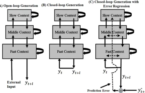
Figure 1: Schemes for (A) open-loop output generation (B) closed-loop output generation (C) closed-loop output generation while inferring the internal states by the error regression.
Parameterlrepresents the number of predicted steps. In (A), by giving current external input, MTRNN generatesl look-ahead prediction steps as outputs. In (B) and (C), by giving the current output prediction (yt), MTRNN generatesl look-ahead prediction steps as outputs (yt+l).
Prediction outputs can be generated in three di↵erent ways. The first called sensory entrainment or open loop generation is a scheme whereby the feeding of
100
perceptual inputs to the network model entrains its internal neural dynamics, enabling predictive outputs. The second way is called closed-loop generation in which the output prediction sequence is generated by copying the current step perceptual prediction in the output units into the next step perceptual inputs.
This operation can be used to generate mental simulation [14, 15] of possible
105
perceptual sequences based on the current intention without using the real per- ceptual inputs from the environment. Schematics of open-loop and closed-loop operations are shown in Figures 1(A) and 1(B). Parameter l in Figure 1 rep- resents the number of predicted steps, i.e. given current input, the MTRNN generatesllook-ahead prediction steps as output. Parameter lwas set as 5 in
110
our simulation experiments and 7 in the robot experiments.
The third way is called closed-loop output generation while inferring the internal states by error regression. This is the main scheme employed in the current paper, enabling on-line action generation via predictive coding. Action is generated along with the top-down prediction of the perceptual sequence in
115
the closed-loop way based on the current internal state representing the intention of the model network. In the other direction, prediction error is generated from the perceived action outcome and the internal state is modified in the
direction of minimizing prediction error via error regression in the bottom-up manner. Further actions are generated based on the modified intention while
120
the top-down and the bottom-up processes iterate in an on-line manner. A schematic of closed-loop output generation while inferring the internal state by error regression can be seen in Figure 1(C).
The learning process of a MTRNN involves the optimization of the ini- tial context states corresponding to all exemplar sequences for the purpose of
125
minimizing prediction/reconstruction error. Variations in initial context states account for di↵erent classes of patterns to be learned and for fluctuations within each class.
2.2. Generation and training methods
Neural unit activation dynamics are those of the leaky integrator neuron as
130
shown in Equation 1.
ut+1i =
✓
1 1
⌧i
◆ uti+ 1
⌧i
0
@X
j
wijctj+X
k
wikxtk+bi
1
A (1)
where uti is the internal state value of the ith neural unit at timet, wij is the connectivity weight from the ith context unit to the jth context unit, wik is the connectivity weight from theithneural unit to thekthinput unit,ctj is the context unit activation value of thejthneural unit at timet,xtk is the external
135
input of thekthinput unit at timet,bi is the bias of theithneural unit, and⌧i
is the time constant of theith neural unit. If the neural unit does not belong to the lowest level sub-network, the second summation term does not exist, since there are no connections to the input units. The context units inside the lowest level sub-network are referred to as Fast Context (FC) units while the
140
ones inside the highest level sub-network are referred to as Slow Context (SC) units. If there are sub-networks between the highest and lowest sub-networks, context units inside them are referred as Middle Context (MC) units. Similar to [5], input and output units are only connected to FC neurons. All output units have a time constant of 1 in this paper.
145
The context unit output values are found with the following activation func- tion as recommended by [16, 17] for faster convergence.
cti= (1.7159) tanh(2
3uti) (2)
The connection weights between context units (wij) are bidirectional (wij 6= wji). If a MTRNN consists of only two sub-networks, all neural units are con- nected to each other. If a MTRNN consists of three sub-networks, no connec-
150
tions between FC and SC units exist (see Figure 1). A softmax transformation is used to remap each inputxtiinto a higher dimensional spacextij according to
receptive fields of adjacent intervals of equal length, as follows [18]:
xtij = exp⇣ ||k
ij xti||2⌘ P
j2Zexp⇣ ||k
ij xti||2⌘ (3)
wherekij represents thejthdimension of the reference vector for theithdimen- sion of the real input value before transformation at timet,xti is the real input
155
value at timet, is a constant value that specifies the shape of the distribution (set as 0.05 in our all experiments), Zis the dimension of the reference vector andxtij is the transformed vector. Zis set 11 in all experiments and it is found heuristically. Sparse encoding of input data is achieved by using the softmax transformation and it can reduce the overlaps of input sequences[5]. In this
160
paper, variables including inputs and outputs before mapping by the softmax transformation or after mapping by inverse softmax transformation are called the real variables and the variables that are mapped by the softmax transforma- tion are called the softmax variables (softmax inputs or outputs). The reference vectors are computed by the equation below:
165
kij=BiM in+BiM ax BiM in
Z 1 (j 1) (4)
whereBiM in,BiM ax, and Zrepresent the minimum value for the ith dimension of the real input data, the maximum value forith dimension of the real input data, and the dimension of the reference vector, respectively.
The activations of the output units are computed as follows:
utij =X
l
wijlctl+bij (5)
ytij= exp utij P
k2Zexp(utik) (6)
whereutij is the internal state of thejth softmax output unit corresponding to theith real output unit,wijlis the connectivity weight from thelthneuron in
170
the FC units to thejthsoftmax output unit corresponding to theithreal output unit,ctl is the context output of thelthneuron in the FC units,bij is the bias of thejth softmax output unit corresponding to the ith real output unit, andytij is thejthsoftmax output unit corresponding to theithreal output unit at time t. The inverse of the softmax transformation described in Eq. (7) calculates the
175
ith dimension of the real output units (yit) at timet. In other words, Eq. (7) maps the softmax outputs to their original dimensions (real outputs).
yti =X
j2Z
ytijkij (7)
A conventional back-propagation through time (BPTT) scheme is used for the network training [19, 20]. The learnable parameters are optimized in the direc- tion of minimization of the Kullback-Leibler divergence (noted as E) between
180
desired (target) and real activation values of softmax output units (¯yti and yit, respectively), according to Equation 8 [5]:
E= XT t=1
X
i2O
yitlog(y¯ti
yti) (8)
WhereTis the length of a sequence. All learnable parameters, shown as✓, are weights and biases and initial states that approach their optimal values in the opposite direction of the gradient @E@✓, and they are updated as follows:
185
r✓(n+ 1) =µr✓(n) ↵@E
@✓ (9)
✓(n+ 1) =✓(n) +r✓(n+ 1) (10)
where↵is the learning rate, set as 0.00003 in all of our experiments, and µis the momentum term which is set as 0.9 in all experiments. These values were found heuristically. The weight and bias gradients for all training sequences (s) can be obtained as follows:
@E
@wij
= (1
⌧i
P
s
P
t @E
@utixtj, (i2C ^ j2I)
1
⌧i
P
s
P
t @E
@utictj, (i2C or O ^ j2C) (11)
@E
@bi
= 1
⌧i
X
s
X
t
@E
@uti (12)
whereC is context units,I is input units, andO is the output units. @u@Et i can be computed using Equation 13:
@E
@uti = 8>
><
>>
:
yit y¯ti, (t 1 ^ i2O) P
j2C @E
@ut+1j [ ij(1 ⌧1
i) +⌧1
iwjic0(uti)]+
P
k2O @E
@utk[wkic0(uti)], (t 0 ^ i2C)
(13)
wherec0(uti) is the derivative ofcti at timet, and is Kronecker delta function.
As learning begins, synaptic weights (wij) are set randomly from a uniform distribution on the interval [N1
I, N1
I] (ifj 2 I) and [N1
C, N1
C] (otherwise), where NI andNC are the number of input and context units, respectively, and biases and initial states are set to 0. The open-loop approach was used in the learning
190
phase in all experiments, i.e. the MTRNN receives current inputs and generates one or multiple look-ahead prediction steps as outputs. Training ran for 50000 epochs in all experiments, and average mean square error (MSE) of closed-loop generation was computed in each training epoch. The learnable parameters obtained from the training epoch with minimum average MSE of closed-loop
195
generation were used in test phases. It should be noted that the closed-loop generation did not a↵ect updating of the learnable parameters.
2.3. Inferring internal states by error regression during synchronized imitation After the learning process, the MTRNN model was tested on a synchronized imitation task. Given target temporal patterns were structurally the same as
200
learned ones, but with modulations in speed and amplitude. During synchro- nized imitation, the model has to imitate the target pattern without delay by predicting next step input by inferring the prototypical patterns to be generated as well as their modulations. The MTRNN does this by using error regression to infer the intention. Closed-loop prediction of target patterns is accomplished
205
by backpropagating prediction error through time (within a temporal window (W) of the immediate past) from the output through the internal states of the MTRNN in a bottom-up manner, thereby modifying internal states in order to minimize the current prediction error. In greater detail, by means of the BPTT scheme the prediction errors from thet-Wtime step to the currentttime step
210
can be used to update the internal states of thet-Wtime step, which result in changes to all context units and prediction outputs inside the temporal window.
It should be noted that the connectivity weights and biases obtained during the learning phase are fixed in the error regression during synchronized imitation testing.
215
Equations used in updating the internal states (activation states of all con- text units in the whole network) at the onset of a temporal window are same as equations 9 and 10. However, we use a di↵erent term for the learning rate (↵) in the error regression scheme. This is called the error regression adaptation rate (↵ER), and was set as 0.001 in all of the present experiments except for the
220
last robotic experiment. Also, we do not use the momentum here (we set the value to zero). In all present experiments, the temporal window length was set to 15 and error regression was performed for 100 regression steps. All former internal states were overwritten from the t-15time step to the current t time step at each time step within the temporal window. By inferring the internal
225
states inside the temporal window, the prediction of internal states and output values after this window (future plans) can be also modified (see Figure 10 for details).
3. Simulation experiments
Two simulation experiments investigated the basic mechanism of the model
230
network in coping with temporally fluctuating patterns. The first experiment examined how the proposed model learns to extract essential dimensions of fluc- tuations latent in exemplar patterns, and how the error regression can utilize the learned structures in successfully performing synchronized imitation. The second experiment examined what sorts of dynamic structures develop in the
235
model during learning naturally fluctuated low dimensional patterns generated by human subjects using a drawing tablet. Analysis suggests that error re- gression with fluctuated patterns employs both the transient and steady state regions. Note that these simulation experiments employed relatively simple patterns without compositionality or hierarchy. Our focus was testing the ex-
240
pectation that the slow dynamics of the higher level of the MTRNN would play
a crucial role in coping with fluctuations in exemplar patterns as well as in the test patterns, so more complex patterns were not necessary.
3.1. A sine-curve pattern with two dimensions of fluctuation
This section reviews a simple experiment using a one-dimensional sine curve
245
as shown in the following equation y=Asin(B⇡
pt), (t 0) (14)
where A, Bare variables that modulate the amplitude and period of the sine curves, andpis set to 30. Training sequences were made in two forms. In the first case, periodicity fluctuation, 5 sine-curve patterns were generated in which each signal had 5 cycles. Only the periodicity of sine-curve patterns was fluctuated
250
(time warped signals). Values ofA were set to 1 for all sequences butBvalues were chosen randomly each cycle from a normal distribution with a mean value (µ) of 1 and standard deviations ( ) of 0.2. This means that 25Bvalues were chosen randomly (each cycle had a di↵erent value). In the second case known as amplitude fluctuation, we generated 5 di↵erent sine-curve patterns by settingB
255
as 1 and choosingAvalues randomly, meaning that only the amplitude of each cycle was fluctuated. One MTRNN referred to as MTRNN-P was trained in order to reconstruct the 5 training patterns with fluctuation in their periodicity whereas MTRNN-A was trained in order to reconstruct the 5 training patterns with amplitude fluctuation. Both MTRNNs consisted of 20 FC, 10 SC, 11
260
softmax input and 11 softmax output units. The time constants of FC and SC units were set to 2 and 50, respectively. Training ran for 50000 epochs in each case.
After training, both MTRNN-P and MTRNN-A successfully regenerated all training patterns in a closed-loop manner by using corresponding initial states,
265
with average mean square error (MSE) of 0.0456 for MTRNN-P and 0.0108 for MTRNN-A. In the test phase, we generated two test patterns using Equation 14 in the same way that we generated training patterns, but with the standard deviations ( ) of these two test patterns set at 0.3. The first test pattern had fluctuations only in its periods while the other had fluctuations only in its
270
amplitudes. The error regression results of MTRNN-P and A are given for the two test patterns in Figures 2 and 3. The first and second rows in both figures show prediction outputs and Mean Square Errors (MSEs), respectively.
Looking at these figures, we can see that both networks show good perfor- mance when they are tested with same dimension of fluctuations as that with
275
which they were trained, while they both generate large errors when they are tested with dimensions of fluctuation di↵erent from their training patterns. In other words, the MTRNN can perform synchronized imitation by minimizing er- ror only with target patterns sharing the same fluctuation structures as learned ones. And thus, error regression enables the network to infer internal states
280
corresponding to currently perceived fluctuations in patterns by way of these prior learned structures.
Figure 2: Closed-loop output generations with the error regression and MSE of MTRNN-P that was trained using time warped teaching sequences when (A) A test pattern with only fluctuations in its periods (time warped) was used in the test phase and (B) A test pattern with only fluctuations in its amplitudes was used in the test phase.
Figure 3: Closed-loop output generations with the error regressions and MSE of MTRNN-A trained using teaching patterns with only fluctuations in amplitude when: (A) A test pattern with only fluctuations in its periods (time warped) was used in the test phase, and (B) A test pattern with only fluctuations in its amplitudes was used in the test phase.
3.2. Naturally fluctuated pattern
The next simulation experiment involves naturally fluctuating patterns in- stead of the computer-generated patterns of the previous experiment. Here,
285
model performance in learning and in synchronized imitation by error regres- sion is demonstrated using low-dimensional temporal patterns, one made by a computer without perturbation, and the other made by a human attempting to mimic the computer generated patterns using a tablet input device. The first type of training pattern was generated using equations for a circle and for
290
Lissajous curves as follows:
(y1=rcos(t) +a1, (0t2⇡)
y2=rsin(t) +b1, (0t2⇡) (15) (y1=A1sin(a2t+ 1), (0t2⇡)
y2=B1sin(b2t), (0t2⇡) (16) where, in Equation 15,r, a1, andb1 were set as 0.4, 0, and -0.2, and in Equa- tion 16, A1, B1, a2, b2 and 1 were set as 0.5, 0.5, 1, 2, and ⇡2, respectively.
Each training pattern consisted of 5 full cycles (tgoes from 0 to 2⇡ in one full cycle) of circle and Lissajous figures. It should be noted that these two training
295
patterns exhibited no fluctuation. They were perfectly regular.
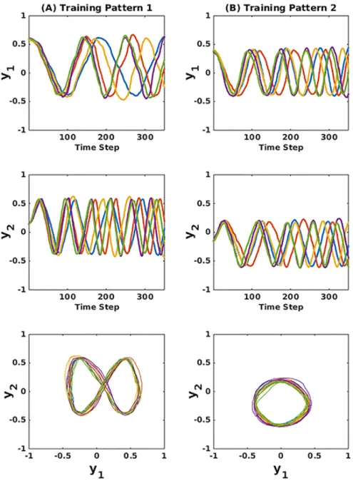
The second type of training pattern was generated by humans attempting to draw the same circle and Lissajous-curve patterns on a drawing tablet. As in the first type, patterns were generated for 5 full cycles for each figure. Two dimensions of fluctuation were naturally generated, both time-warping and am-
300
plitude shifting, as illustrated in tablet generated training pattern 1 and 2 in Figure 4(A) and Figure 4(B), respectively. The first and second rows show the first dimension (y1) and second dimension (y2) of training patterns over time.
Their phase plots appear in the third row. The 5 Lissajous-curve patterns shown in Figure 4(A) di↵er in periodicity and amplitude. The same is evident in the
305
circle-curve patterns in Figure 4(B). See Figure in Appendix B for computer generated patterns.
One MTRNN referred to as MTRNN-C (using computer generated patterns) was trained to reconstruct the 2 computer-generated training patterns (as in the first experiment) and another MTRNN referred to as MTRNN-H (using human
310
generated patterns) was trained to reconstruct 10 naturally generated training patterns. Both MTRNNs consisted of 30 FC, 15 SC, 22 softmax input and 22 softmax output units. The time constants of FC and SC units were set to 2 and 50, respectively. The training was successfully done for 50000 epochs for both cases.
315
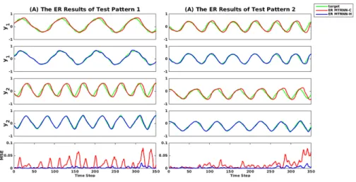
In the test phase, the two test patterns, one Lissajous-curve pattern (test pattern 1) and one circle-curve pattern (test pattern 2), were generated by drawing tablet. Then, we looked at how the error regression exploits the learned structures in performing synchronized imitation with these two target patterns.
Error regression results are depicted in Figure 5. The first and second rows
320
show the first (y1) dimension of the error regression outputs and target patterns
Figure 4: Training patterns generated by a human using a drawing tablet when (A) 5 Lissajous-curve patterns were produced and (B) 5 circle-curve patterns were produced. The first and second rows illustrate the first (y1) and second (y2) dimensions of the patterns, respectively. The last row shows the phase plots of training patterns 1 and 2.
Figure 5: Comparison of closed-loop output generations with the error regression and MSEs for MTRNN-C that was trained using computer generated patterns with no fluctuations and for MTRNN-H that was trained using naturally fluctuated patterns given (A) Lissajous-curve pattern (test pattern 1) and (B) Circle-curve pattern (test pattern 2). ER MTRNN-C and ER MTRNN-H are abbreviations for the error regression outputs of MTRNN-C and the error regression outputs of MTRNN-H, respectively. The first and second rows show the first di- mension of ER outputs and target patterns for MTRNN-C and MTRNN-H, respectively, while the third and fourth rows illustrate the second dimension of ER outputs and target patterns for MTRNN-C and MTRNN-H, respectively. The green, red, and blue lines correspond to test target, ER MTRNN-C and ER MTRNN-H, respectively.
for MTRNN-C and MTRNN-H, respectively, and the third and fourth rows illustrate the second (y2) dimensions of the error regression outputs and target patterns for MTRNN-C and MTRNN-H. The red and blue lines in the last row represent MSEs for MTRNN-C and MTRNN-H, respectively. This figure shows
325
that MTRNN-H outperforms MTRNN-C. It can be also seen that the proposed model can deal with time-warping and amplitude shifting which were naturally generated inside the test patterns.
As explained earlier, for each training pattern, the MTRNN learned initial context states during the leaning phase. By using the initial states correspond-
330
ing to 2 training patterns of MTRNN-C, closed-loop output generations were computed for 50000 time steps. Likewise, by using initial states corresponding to 10 training patterns, MTRNN-H closed-loop output generations were com- puted for 50000 time steps. The phase plots for the first and last 4-cycle of the closed-loop output generations of MTRNN-C for the first pattern (Lissajous-
335
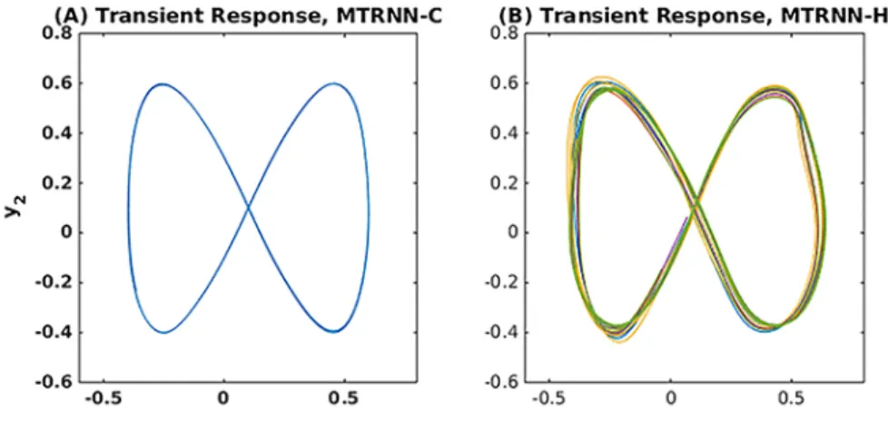
curve pattern) are shown in Figure 6(A) and Figure 6(C), respectively. Sim- ilarly, the phase plots for the first and last 4-cycle of the closed-loop output generation of MTRNN-H for the first patterns (Lissajous-curve patterns) are depicted in Figure 6(B) and Figure 6(D), respectively. The first and last 4-cycle responses are referred to as transient and steady-state responses, respectively.
340
It should be noted that in both Figure 6(A) and Figure 6(C), the transient and steady-state closed-loop output for only one pattern are shown because only one Lissajous-curve pattern was included in the training phase of MTRNN-C. Fig- ure 6(B) and Figure 6(D) illustrate the transient and steady-state closed-loop output generated for 5 patterns because there were 5 Lissajous curve patterns
345
in the training phase of MTRNN-H. It is also worth noting that the same results were obtained for circle-curve patterns that are not shown here.
In Figure 6, it can be seen that MTRNN-C learns a given target pattern as a global attractor, and the transition from the adapted initial states is quite short when compared to that of MTRNN-H. MTRNN-H encodes the trajectory of an
350
averaged target pattern among multiple fluctuated patterns as a global attrac- tor, and fluctuated patterns outside of the averaged pattern are reconstructed in the larger transient region.
Principle Component Analysis (PCA) was used to visualize the slow context activities of MTRNN-H in both training and test phases. PCA was applied on
355
the corresponding slow context activities of the closed-loop output generations shown in Figures 6(B), and 6(D), and the first and second principle components are shown in Figure 7(A). The 5 patterns have di↵erent slow context activities in the transient region, but they all have the same activities in the steady- state region, consistent with results shown in Figures 6(B) and 6(D). PCA was
360
also used to visualize the slow context activities of the error regression with test pattern 1 (corresponding to ER MTRNN-H in Figure 5(A)), and the first and second principle components are shown in Figure 7(B). The same steady- state figure shown in Figure 7(A) is repeated in Figure 7(B) to facilitate the visualization.
365
Figure 7(B) shows that the error regression moves between the steady state and transient regions, with most activity within the transient region. Comparing
Figure 6: This figure illustrates the transient closed-loop output generations of (A) MTRNN-C and (B) MTRNN-H and also the steady-state closed-loop output generations of (C) MTRNN- C and (D) MTRNN-H for all Lissajous-curve training patterns. The closed-loop output gen- erations were computed for 50000 time steps by using the initial states of all training patterns that were obtained in the learning phase. The first row (transient response) show the phase plot of the closed-loop output generation in the first 4 cycles, which are almost the same as corresponding training patterns shown in the last row of Figure 4. The second row shows the phase plot of the closed-loop output generations in the last 4 cycles (from time step 49500 to 50000) referred as the steady-state response.
Figures 7(B), 6(B) and 6(D), it can be seen that fluctuated patterns are learned in the transient region, and that the error regression can infer both this transient region and steady-state regions through modulation of internal states.
370
4. Robot experiments
Imitation learning, which is called also learning by observation, has been widely studied in di↵erent fields of research. In robotics, imitation learning has been approached in terms of symbolic reasoning [21, 22, 23] and non- symbolic learning tools such as fuzzy logic [24], the Active Intermodal Matching
375
(AIM) mechanism [25], Dynamical Recurrent Associative Memory Architecture (DRAMA) [26], and the MTRNN [27]. These models have allowed robots to follow and to learn multiple skills and actions from their tutors. For example, in an imitation game between a human and robot using a RNNPB model without hierarchy [6], the model was first trained to memorize multiple cyclic movement
380
patterns of a human subject and was then used to control a robot in the re- generation of the memorized patterns. However, this study did not examine the problems introduced with pattern fluctuation. Many graphical probabilistic models such as hidden Markov models have been used to overcome the problem of fluctuation in temporal patterns such as the time-warping problem [28, 29, 30].
385
The present study attempts to show that the proposed RNN models can also deal with this problem by using its dynamical systems characteristics. In fact, RNNs work better for storing and accessing information over long periods of time than conventional sequential pattern learning algorithms such as hidden Markov models [31].
390
As explained in previous sections, the MTRNN is able to cope with fluctua- tions such as time warping and amplitude shifting during simple tasks. To test our model in more realistic situations, we conducted two robotic experiments involving imitative interaction between a humanoid robot and human subjects.
These experiments examined how the proposed model can support spontaneous
395
interaction between robots and human subjects while dealing with possible fluc- tuations in perceived temporal patterns. The first experiment follows human subjects in acquiring a set of cyclic patterns also learned by the robot during an imitation game. Synchronized imitation can be achieved on the robot side by using the on-line error regression of the internal states within the window of the
400
immediate past. Natural interaction forces the robot to deal with more naturally fluctuated patterns. The second experiment examined how the balance between the top-down intentional process from the higher level and the bottom-up recog- nition processes from the lower level can a↵ect spontaneous interaction between the robot and the human subjects by changing the error regression adaptation
405
rate (↵ER). These robotic experiments employed a larger MTRNN than those used in the previous experiments consisting of three sub-networks, one with fast dynamics, one with intermediate dynamics and one with slow dynamics for the purpose of coping with more complex patterns (such as the hierarchically organized movement patterns used in the second robotic experiment).
410
Figure 7: Slow context activities in a 2 dimensional space based on the results of PCA analysis. (A) Shows the slow context activities of the transient and steady-state closed-loop output generations of 5 training patterns corresponding to Figures 6(B), and 6(D). (B) shows the slow context activities of the error regression for test pattern 1 corresponding to ER MTRNN-H in Figure 5(A). Transient responses of slow context activities (the first 4 cycles) of the training patterns 1 to 5 are indicated by transient1 to 5 (dotted lines) in (A). The steady- state dotted line (pink dotted line) in (A) shows the steady-state responses of slow context activities (the last 4 cycles) of training patterns 1 to 5. Only one line appears because all 5 steady-state responses are the same and so perfectly overlap. In (B), test pattern 1 shows the slow context activities of the error regression with test pattern 1 and the same steady-state results shown in (A) is repeated here again in order to aid visualization.
Figure 8: (A) Schematics of the direct method and (B) three cyclic movement patterns. MP is the abbreviation for movement pattern. The direct method is used during training and the MTRNN is not used for controlling the NAO. With the direct method, three movement patterns shown in (B) were generated.
4.1. Robot experiment design
We employed a NAO humanoid robot (developed by Aldebaran Robotics) and a Kinect sensor (developed by Microsoft) for imitative interaction tasks.
The Kinect SDK and OpenNI framework were used to track the 3-D (X, Y, Z) coordinates of a humans arm joints. The 3-D positions of human-user arms
415
were mapped to the 3-D positions of the NAO’s arms with respect to the robot coordinate system. Next, the 3-D positions of the NAO were mapped to its joint angles (shoulder roll, and pitch and elbow roll, and yaw) by applying inverse kinematics.
4.2. Imitative interaction game
420
We designed an imitative interaction game between a robot and human subjects in order to investigate how well the model could cope with naturally fluctuated patterns generated by human subjects.
First, training data were collected by the experimenter who interacted with the NAO using the direct method. The direct method refers to the situation
425
where a MTRNN is not used to control the NAO as shown in Figure 8(A).
The three cyclic movement patterns shown in Figure 8(B) were generated using only the shoulder roll and pitch of both arms. Other joint angles remained fixed.
Similar to Section 3.2, 5 sequences of training data were collected for each cyclic movement pattern. The final 15 training patterns had average time lengths of
430
232 steps with each time step length lasting 75 ms. There was around 520 ms delay between actual human movement patterns and perceiving them by the
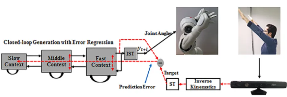
Figure 9: Schematic of the imitative interaction game. ST and IST are the abbreviation for softmax transformation and inverse softmax transformation, respectively. The 4 joint angles that are obtained after the inverse kinematic are mapped by softmax transform to be used as targets in the error regression process. The softmax outputs are then mapped to real outputs (joint angles) through inverse softmax transformation.
Kinect sensor. To overcome this delay, the prediction steplwas set to 7 in all robotic experiments (7*75=525 ms).
A MTRNN consisting of 30 FC, 20 MC, 10 SC, 44 softmax input and 44 soft-
435
max output units was trained to reconstruct these 15 cyclic movement patterns.
The time constants of FC, MC, and SC units were set to 5, 25, and 150, respec- tively. The training was successfully performed for 50000 epochs. The trained MTRNN was used in an imitative interaction game using the error regression approach as shown in Figure 9. 10 university students participated in the ex-
440
periment, in which they interacted with the NAO without any prior knowledge about the cyclic movement patterns and experiments. Their first task was to figure out all of the movement patterns memorized by the MTRNN while achiev- ing synchronized imitation with the NAO. This was a challenging task because human subjects tried so many di↵erent patterns with di↵erent periodicities and
445
amplitudes in order to figure out the memorized patterns. They were given 10 minutes for the first trial, but if they failed to figure out all 3 movement patterns, they could have another trial with duration of 5 minutes. If again the human subject failed, he/she was given another 5 minutes. It turned out that all participants were able to interact with the NAO successfully. However, two
450
of them could not figure out one of the movement patterns.
The second task for the human subjects was to synchronize with the robot.
First, they had to repeat movement pattern 1 until they felt that they were well synchronized with the NAO, then they could switch to movement pattern 2 and do the same, and finally they could synchronize movement pattern 3.
455
All subjects synchronized successfully with the NAO. Previous and current task results show that the network deals with time warping and amplitude shifting even in such a noisy natural environment.
Figure 10 displays the detailed dynamic of the error regression approach for one of the participants during the synchronization stage. In Figure 10(A),
460
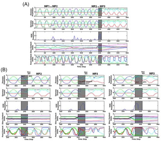
Figure 10: Detailed dynamic of the error regression scheme for one of the participants during the synchronization stage. Plot (A) illustrates error regression results during a large period of time (from 0 to 500). (B) shows error regression results during a shorter period of time (from 300 to 400) and the regression dynamic is shown for three di↵erent current (Now) time steps;
347, 355, and 363 referred to as the pre-modification, modification and post-modification phases, respectively. The gray areas are the temporal windows of the immediate past in which the internal neural states are modified to minimize the error. Changing states inside the temporal window can also a↵ect future states, but states before the temporal window cannot be changed. As shown in left panels of (B), the plan is di↵erent from the sensory target, which is why a large MSE is generated in the pre-modification phase. The slow and fast context states are modified by error regression, and the plan is changed in the modification phase (MP3). As a result, MSE decreases significantly and sensory predictions follow the target in the post-modification phase. The blue, red, green, and cyan lines correspond to right shoulder pitch, right shoulder roll, left shoulder pitch, and left shoulder roll, respectively. A video corresponding to this figure can be seen in Appendix A
transitions from movement patterns 1 to 2 (M P1 ! M P2) and from 2 to 3 (M P2 ! M P3) are shown at the top of the sensory prediction (sensory output) panel. The temporal windows of the error regression at a particular moment of switching from movement pattern 2 to 3 are depicted by gray areas in all panels, with the current time (labeled as now in Figure 10(B)) indicated
465
in the right line of the windows. Internal states cannot be modified before the temporal window, but they can be revised within it to minimize prediction error by means of BPTT. Predicted states after this temporal window (the plan) are obtained by continuing closed loop generation to the end for each time step.
The error regression procedure can be seen more clearly in Figure 10(B).
470
Sensory inputs, their prediction and the internal states change from the time step 300 to 400. The states for the current time steps (now) of 347, 355, and 363 are so-called pre-modification, modification, and post-modification phases, re- spectively. In the pre-modification phase depicted in the left panels, the human subject starts to change the movement patterns from 2 to 3 and MSE increases.
475
The plan is still the movement pattern 2 (MP2) at this point. During the modi- fication phase shown in the center panels, neural internal states in both SC and FC units are revised by error regression in order to reduce prediction error, and change the intention state. The immediate past of states is changed inside the temporal window and the plan is changed to movement pattern 3 (MP3), and
480
remains movement pattern 3 in the post-modification phase displayed on the right panels. The MSE decreases significantly in the post-modification phase and the sensory prediction follows the target. Pre-modification, modification, and post-modification phases demonstrate that both future predicted states and the record of past states di↵er from each other during the same time steps. This
485
is because during each time step, immediate past states within the temporal window can be overwritten by means of error regression, thereby modulating internal neural states. Past states outside of the temporal window are constant and cannot be changed by error regression, however.
We also compared the performance of the error regression scheme with that
490
of the conventional sensory entrainment scheme (open-loop output generation) using the same MTRNN. In other words, we did not use the error regression scheme, instead inputting directly to the sensory inputs of the MTRNN from the Kinect. The test experiment showed that it was difficult for the robot to synchronize with human movement patterns using the entrainment scheme. The
495
sensory entrainment scheme is not powerful enough to immediately modify the internal states in order to minimize prediction error. Also, we tested a case in which error regression was applied to SC units but not to FC units, analogous to the on-line adaptation of PB units in previous work [6]. It was again found that synchronization between the human subjects and the robot was not easily
500
achieved.
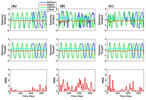
In order to show quantitative di↵erences between these three schemes, we conducted an o↵-line synchronized imitation test using a test sensory pattern containing sequential switching between two trained prototypical patterns. The test pattern was collected by using the direct method. The simulation results
505
are shown in Figure 11. The left panel shows the results of the proposed model.
Figure 11: The sensory output, sensory target, and MSE results of (A) The error regression scheme, (B) The error regression scheme when only SC internal neural units are modified, and (C) Sensory entrainment scheme. The RSPitch, RSRoll, LSPitch, and LSRoll abbreviate right shoulder pitch, right shoulder roll, left shoulder pitch, and left shoulder roll, respectively.
Joint angles are measured in radians.