山形県立米沢女子短期大学
『生活文化研究所報告』
第47号 抜刷 2020年3月
from the Students’ Perspective
伊豆田 義人
IZUTA Giido
Assessing Regional Depopulation Measures from the Students’ Perspective
伊豆田 義 人
IZUTA Giido
Abstract
The goal of this investigation is to assess from the students’ perspective some of the current countermeasures to cope with the relocation of young people from countryside Japan to metropolitan areas after finishing college.
Basically, the field work took place in a typical middle scale city facing depopulation in the northeastern region of Japan with a population of 85,000 people, long winters and relatively heavy snow during the cold season. College students residing in this city were asked to participate in a survey research to evaluate five topics expressing some potential measures to cope with the young people’s moving out to big cities after graduating college. Each topic was composed by several attributes, in which some of the countermeasures are currently being implemented by policy makers. Students were asked to evaluate, according to a 5 point scale, the level of effectiveness of these attributes in making them settle down in the countryside. The statistical analysis on the basis of the confirmatory factor analysis was performed to generate a model, which showed that topics ‘settling down support system’ and ‘shopping options’
depend on the other topics, meaning that students give priority to the latter - namely, ‘job availability’, ‘metropolis- oriented opportunities’, and ‘financial support system’ - and will rather establish in the countryside as long as their composing attributes are fulfilled first. Finally, these findings allow us to understand what college graduates are aspiring after going out of college. They also provide countryside governments some basic data to help them cope with the depopulation issues.
Key words: Relocation to Metropolis, Rural Areas issues, Regional Depopulation, Statistical Model, and ‘Kasoka’.
1. INTRODUCTION
The regional depopulation phenomenon is called ‘kasoka’ in Japanese and refers to a chronic decline in the number of population of a certain geographical area or municipality due to factors as relocation of young people from their hometowns to big cities and surrounding areas, and dwindling birthrate combined with aging population. Actually, the Japanese government has since long established some standard quantitative parameters in order to be able to identify whether a local municipality is in ‘state of kasoka’ (Takafumi, 2010; MIC, 2016a). This procedure started with the enactment of the ‘Law Concerning Emergency Measures for Underpopulated Areas’ in 1970, which has been revised and updated every ten years. In fact, the current law, which was endorsed in 2010 and is under effect until the year 2020, provides some definitions of ‘state of kasoka’ on a case-by-case basis according to the characteristics of the area, with the simplest requirement being that the municipality underwent a decrease in the number of population of more than 33% over the last 45 years, a period spanning from 1965 to 2010. Furthermore, according to some statistical data, the number of rural towns and cities in ‘state of kasoka’ sums up to a little less than 800 as of 2016 (Kaso-Net, 2016).
A detailed analysis of the demographic distribution and temporal transition in Japan can be found in Matanle’s work (Matanle, 2014), which includes discussions on the future consequences of the regional depopulation on the domestic and global economies as well as policies in all levels of public administration whether central or regional. In
the early days when this massive efflux of young people from provincial to metropolitan areas matters just began to be dealt with as a long run administrative challenge, researchers focused mainly on the human relocation as the main cause of ‘state of kasoka’, and studied intensively the social and economic impacts of some of the major variables associated with this phenomenon as lack of labor shortage in big cities during the post-war Japanese rapid economic growth on the regions (Takeuchi, 1974; 1976). If the reality itself has not changed a lot since then, at least, the social issue itself has become far more serious with alarm bells for some new agenda concerning the high concentration of population in megalopolis being rung from all directions; not to mention that nowadays the depopulation problem is also closely related to other social aspects, among them the fast aging population and low birth rate as previously mentioned (Kato, 2014).
Apropos, relying on these backgrounds, the authors have in recent years investigated the depopulation phenomenon in the northeastern areas of Japan through the mind of young regional people by exploring their world and their attitudes towards choosing a place as their future local of residence. In fact, a conjoint analysis model of a possible social model composed by variables as big cities, rural towns, and deliberate relocation of individuals from rural to urban areas at their entrance to the workforce was pursued in order to study the relationships between the depopulation in the northeast countryside and the social perceptions as well as the imaginary picture that the young people draw of these urban areas as residential location (Nakagawa & Izuta, 2016; Izuta, Nakagawa, Nishikawa, &
Sato 2016). Then, this quantitative model was further refined to embrace their values like the craving for the latest fashion and daily life goods; instant access to real time news, gossips, and entertainment buzz; and the feeling that they are part of a huge, 24/7 never-stopping dynamic and lively metropolis (Izuta, Nakagawa, & Tanaka, 2017a).
The model components were to some extent underpinned by a companion research on the attitudes of youths towards their countryside hometowns, in which some environmental factors as urban size and economic development, as well as psychological elements including the longing for living in a big city are picked up to assess the fulfilling urbanity feeling that they have of the countryside in the sense that they would feel equally better off - or somehow come reasonably well to terms with - living in the countryside as anywhere else in a big city (Izuta, Nakagawa, & Tanaka, 2017b). In addition, factors related to urban and social developments - among them, the improvement and expansion of city infrastructures, some free medical assistance services for infants under certain age, and elderly friendly living environment - that are being implemented in some municipalities were also considered and a statistical model was generated out of the exploratory factor analysis (Izuta, Nishikawa, Nakagawa, & Abe, 2018a; 2018b; Izuta, Nishikawa, Nakagawa, & Hanazumi, 2018).
This paper aims to shed some light on the potential causes of the regional depopulation problem from the students’
perspective. To accomplish it, we look into how some local government countermeasures to deal with the outflow of young people from regional areas to metropolises affect college students in their decision to whether or not to establish in a countryside city with a population of about 85,000 people, which is basically a typical middle sized municipality in the northeastern region composed by six prefectures. Note that a prefecture is an administrative unit corresponding to a ‘state’ in some western countries, and sometimes mistakenly referred to as ‘province’, which is a holdover term from the old past era. It is also worth noting that some of these counteractions are not yet put into practice; these were however evaluated because they came up as potential counter-steps during our preliminary studies. Yet, this city was selected due to the following reasons: (1) it is about 1 hour by train, which is equivalent to approximately 70 km far from the capital of the prefecture; (2) it is located about 2 hours far from the biggest city in the region with one million inhabitants; (3) the area is located in a valley with relatively heavy snow falls in winter; (4) Nevertheless it is a college town with the economy largely sustained by its industrial zone, the population has sensitively declined over the past decade at a rate of hundreds of residents per year on average. The research work consisted of basically the collection of data through field work, whose main task was the surveying of college
students, followed by the statistical modeling of the data relying on the structural equation model (SEM) analysis.
Finally, this paper is organized as follows. The details of the experimental procedures are described in section
‘Methodology’; and the results are given in section ‘Results’. Discussions and final comments are presented in the last two sections, respectively.
2. METHODOLOGY 2.1 Sampling and Survey
The investigation was carried out in a city surrounded by mountains and located in the northeastern region approximately 300 km far from the megalopolis Tokyo and 130 km from the biggest city of the region, Sendai City, which has a population of over one million people and is classified according to the population and economic situation as ‘a city designated by ordinance’ by the central government - in plain terms, it gives the city the status of a regional metropolis.
The city chosen for our field work is ranked fourth in its prefecture, with about 85,000 inhabitants, and roughly 50 km far from the capital of the prefecture, which has a population of 240,000 people and has been classified as ‘mid- level city’. Furthermore, the city has four higher education institutions, which help it have a youthful atmosphere of a typical college town found anywhere else in a metropolis. Economically, the city is based on the high tech electronics industry and farming, whereas environmentally, it is characterized by somewhat long and relatively heavy snow during the winters with blizzards sometimes piling up amounts of snow as much as 100 cm depth in just a couple of days.
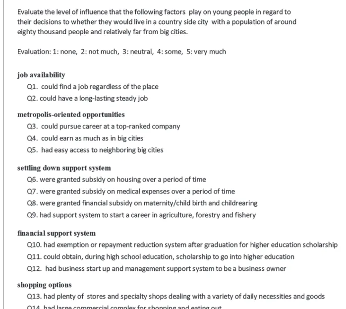
Taking this region as our field of investigation, we first obtained permission from the teachers of a women’s junior college to perform the survey during their classes, then asked students to cooperate voluntarily with our survey. In all, 208 fresh and sophomore female students, aged 18-20 years old, answered to the questionnaires, which in addition to basic personal information as age and city of birth, comprised 14 factors (measured variables) to be evaluated on a 5 point scale basis with the rank 1 (none) meaning that the factor has no influence whatsoever on their decision to whether or not they will settle down in the city, and rank 5 (very much) expressing that the factor has a very strong influence on their decisions. Note that the survey sheets were handed-out and handed-in in the first 30 minutes of the class, and only those who consented to the objectives and the use of their data for research purposes took part in this task.
In addition, since we aim in this work to build a model out of the structural modeling analysis, these 14 factors were selected based on our previous research, and in such way that they can be classified into five groups; namely,
‘job availability’, ‘metropolis-oriented opportunities’, ‘settling down support system’, ‘financial support system’, and
‘shopping options’. These groups are in fact nothing else than the ‘factors’, or latent variables that are generated by the factor analysis framework. Figure 1 shows the main part of the survey sheet.
2.2 Data Processing
Visual checking of each of the 208 collected answer sheets came out with 8 sheets with some unanswered questions or multiple marks for the same questions. Thus, since these were considered invalid answers and excluded from further data processing, this paper is built on the findings achieved out of 200 respondents. The basic personal info and ratings of the factors were first tabbed with computer application Microsoft Excel 2016 running on a personal computer equipped with the OS Microsoft Windows 10. The file was subsequently imported into the statistical freeware R 3.5.1 (R Core Team, 2018) which had the package ‘psych’ (Revelle, 2018) and ‘lavaan’ (Rosseel, 2018) added in its library in order to be able to perform the factor analysis and structural equation modeling.
3. RESULTS
In this section, we present the results of the data processing, starting with the descriptive statistics, which is followed by the factor analysis that is used to verify the initial grouping of the 14 factors (measured variables) evaluated in the survey. Then, the results of the structural equations modeling analysis is presented.
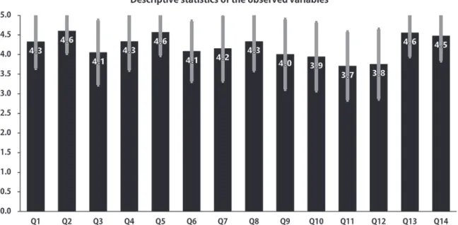
Figure 2 shows the descriptive statistics of the data. As seen in the chart, the variables with the biggest mean value, which is marking 4.6, are ‘Q2. could have a long-lasting steady job’, ‘Q5. had easy access to neighboring big cities’, and ‘Q13. had plenty of stores and specialty shops dealing with a variety of daily necessities and goods’. These are followed by ‘Q14. had large commercial complex for shopping and eating out’ alone, which scored 4.5 on average.
Note that ‘Q10. had exemption or repayment reduction system after graduation for higher education scholarship’,
‘Q11. could obtain, during high school education, scholarship to go into higher education’, and ‘Q12. had business startup and management support system to be a business owner’ recorded below the rank 4 (standing for ‘some’).
Fig. 1: Main part of the survey sheet, which contains 14 factors to be assessed on a five point evaluation basis. The classes ‘job availability’, ‘metropolis-oriented opportunities’, ‘settling down support system’, ‘financial support system’, and ‘shopping options’ translate into the factors (latent variables) in the factor analysis framework.
Fig. 2: Descriptive statistics of the measured variables. N=200. The bars express the mean value of the ratings and the error bars atop stand for the standard deviations of the ratings, which are as follows: Q1=0.67, Q2=0.57, Q3=0.83, Q4=0.73, Q5=0.59, Q6=0.77, Q7=0.83, Q8=0.75, Q9=0.89, Q10=0.87, Q11=0.87, Q12= 0.89, Q13=0.61, and Q14=0.63.
Next, the factor analysis was accomplished in order to check the original classification of the measured variables.
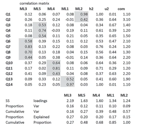
Figure 3 depicts the results of the factor analysis executed on package ‘psych’ by typing the command line ‘fa(r=Data, nfactors=5, rotate="varimax", fm="ml")’, which means that we specified from the very beginning for the number of factor be five as in the setup of the survey.Yet, “varimax” method is used to rotate the factors, and the factoring method (fm) used was maximum likelihood (ml).
Now setting the standardized loading value of 0.40 as a reference and grouping the measured variables, we obtain a model with five factors indexed as ML1, ML2, ML3, ML4, and ML5 with the cumulative variance pointing at 57%; the root mean square of the residual (RMSR), 0.03; the empirical chi-square, 41.98; Fit based upon off diagonal values, 0.99; RMSEA index, 0.077; and Tucker Lewis Index of 0.881. Even though not all of these parameters meet strictly the values of ‘a good model’ as cited in for example (Prudon, 2015), it is still fair to say that their relative close proximity supports the model if we take into account that multiple R square of scores of factors are greater than 0.70, which is also an important parameter when evaluating the validity of the overall model.
In this model, ML1 is related to the measured variables ‘Q13. had plenty of stores and specialty shops dealing with a variety of daily necessities and goods’, and ‘Q14. had large commercial complex for shopping and eating out’;
so it corresponds to the theoretical group ‘shopping options’. Following this reasoning, ML2 reads ‘job availability’;
ML3 translates into ‘settling down support system’; ML4 into ‘financial support system’; and ML5 turns to be
‘metropolis-oriented opportunities’.
Note also that the multiple R square of scores in decreasing order are as follows: 99% of‘ job availability’, 98%
of ‘shopping options’, 79% of ‘settling down support system’, 75% of ‘financial support system’, and 70% of
‘metropolis-oriented opportunities’.
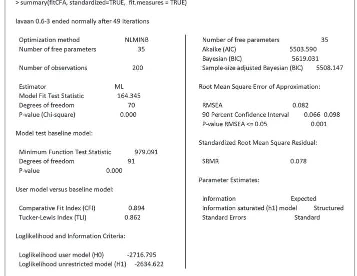
Once the factor analysis substantiated the hypothesized model, we moved on to the structural equations modeling, which was performed with the package ‘lavaan’ as illustrated in Fig.4. As in the factor analysis, the ‘Estimator’
parameter is maximum likelihood (ML). This model has 70 degrees of freedom and p-value (chi-square) was so infinitesimally small a number that it is shown truncated to zero, similar to p-value in the model test baseline model
parameter.
Looking at the indices in the user model versus baseline model section, we see that the comparative fit index (CFI) is 0.894; and Tucker-Lewis Index (TLI) is 0.862. Besides, root mean square error approximation (RMSEA) scored 0.082; p-value RMSEA marked 0.001; the standardized root mean square residual (SRMR) numbered 0.078. If we compare these values with ideal number as found in the literature (Hox, & Bechger, 1998), we see that most of the parameter fall a bit short of the reference. For example, an ideal model is expected to show off TLI and CFI above 95% (0.95). However, in practice these ideal standards are seldom met, unless we have very particular cases whose model components and structure are well-known. In this work, we take for granted that CFI and TLI with values anything greater than 85% (0.85); and RMSEA and SRMR less than 10% (0.1) endorse a practical model.
As a matter of fact, the result of structural equation modeling after some adjustments is as drawn in Fig.5.
Here, the model is composed by two dependent variables, namely those given by common latent variables ML1 (‘shopping options’) and ML3 (‘settling down support system’) revealing that they derive straightforwardly from the latent variables ML2 (‘job availability’), ML3 (‘settling down support system’), and ML5 (‘metropolis- oriented opportunities’), which are the independent variables of the model. Of noteworthy is the fact that ML2 (‘job availability’) and ML5 (‘metropolis-oriented opportunities’) are mutually-correlated, so that there is no cause-and- effect relationship between them, and each define a smaller model that expresses not only the students reasoning, but also the priorities that they feel they need to fulfill. Simply put, dependent variables come after and once the independent variables are achieved. On the other hand, the mutually correlated variables here are the starting point and the ‘game changer’ in the process of deciding whether or not to establish in a specific location.
In a bit more mathematical settings, these latent variables are expressed by a set of equations, which in this case are written as ML3 = 0.76xML4 + 0.26xML2 + e43; ML1 = 0.63xML5 + e51; and ML4 = 0.57xML2 + e24;
provided that e43, e51, and e24 are the exogenous variables, which are basically the errors. The dashed arrowed lines linking the latent variables and the observed variables Q1, Q3, Q9, and Q12 indicate that the errors inherent to the measured variables have factor loadings stronger than those between the latent and measured ones. In fact, the factor loadings of the errors of Q1, Q3, Q9, and Q12 are 0.68, 0.58, 0.56, and 0.58, respectively; whereas the ones between Q1 and ML2 is 0.57; Q3 and ML5 is 0.58; Q9 and ML3 is 0.56; and Q12 and ML4 is 0.58.
4. DISCUSSION
As shown in Fig.3, the factor analysis model supports the survey design given in Fig. 1, in which it was assumed that the common factor ML2 (‘job availability’) explains fairly well the variances of the observed variables Q1 (‘could find a job regardless of the place’) and Q2 (‘could have a long-lasting steady job’). Similarly, ML5 (‘metropolis-oriented opportunities’) makes up a common factor for Q3 (‘could pursue career at a nationwide top- ranked company’), Q4 (‘could earn as much as in big cities’) and Q5 (‘had easy access to neighboring big cities’);
ML3 (‘settling down support system’) for Q6 (‘were granted subsidy on housing over a period of time’), Q7 (‘were granted subsidy on medical expenses over a period of time’), Q8 (‘were granted financial subsidy on maternity/
child birth and childrearing’) and Q9 (‘had support system to start a career in agriculture, forestry and fishery’); ML4 (‘financial support system’) for Q10 (‘had exemption or repayment reduction system after graduation for higher education scholarship’), Q11 (‘could obtain, during high school education, scholarship to go into higher education’) and Q12 (‘had business start-up and management support system to be a business owner’); and ML1 (‘shopping options’) for Q13 (‘had plenty of stores and specialty shops dealing with a variety of daily necessities and goods’) and Q14 (‘had large commercial complex for shopping and eating out’).
On the other hand, the structural equation modeling analysis generated the model depicted in Fig.3 suggesting that the dependent variable ML3 (‘settling down support system’) could be explained by independent variables
Fig. 3: Output of the factor analysis performed with command line ‘fa’.
ML2 (‘job availability’) and ML4 (‘financial support system’), meaning that variables like ‘granted subsidy on housing over a period of time’, ‘granted subsidy on medical expenses over a period of time’, and ‘granted financial subsidy on maternity/child birth and childrearing’ would come after the urge for guaranteed employment and some sort of outlook for either repaying borrowed loans for higher education expenses or means of sustaining their academic education. Yet, the fact that the coefficient of ML4 is greater than that of ML2 suggests that the long-term repercussion of the costs of a professional formation, which not rarely lasts for many years after finishing college and entering the work force, would probably have a stronger influence on the youth willingness to establish in a countryside town.
Furthermore, given that ML1 (‘shopping options’) is explained by the independent variable ML5 (‘metropolis- oriented opportunities’), it is fair to say that the non-fulfillment of the demands for opportunities like ‘career at a nationwide top-ranked company’, ‘earn as much as in big cities’, and ‘had easy access to neighboring big cities’
are to some extent the factors generating the ‘shopping options’ expectations. Interestingly, the descriptive statistics exhibited in Fig. 2 showed high ratings for measured variables Q13 (‘had plenty of stores and specialty shops dealing with a variety of daily necessities and goods’) and Q14 (‘had large commercial complex for shopping and eating out’), which are connected to the independent variable ML1.
The structural equations model also implies that there are two sub-models acting on their decisions to whether or not they would stay in the city. As previously mentioned, the starting point of these models are ML2 and ML5, and
Fig. 4: Output of the structural equations modeling analysis performed with package ‘lavaan’.
these entry points are bi-directionally linked. That is to say, the students would not mind staying in the countryside as long as they could earn as much as in a metropolis. We can see that this assertion holds if we note that nevertheless Q3 (‘could pursue career at a nationwide top-ranked company’) is also correlated to ML5, the loading factor of the error component is greater than the link between ML5 and Q3; and recall that Q5 (‘had easy access to neighboring big cities’) is not related to ML5, but its average rating was one of the highest. In other words, we are solely left with the analysis and interpretation of the relationship between Q2 (‘could have a long-lasting steady job’) and Q4 (‘could earn as much as in big cities’).
5. FINAL COMMENTS
The findings of this study put in the other way around says that creating jobs and opportunities to work for young people is indeed a good approach to deal with the depopulation in the countryside, as in fact many local governments are currently tackling it. However, the structural equations model also shows that the creation of new jobs alone is not sufficient, because the students expect to earn wages equivalent to the ones paid in big cities. In fact, comparing the official minimum wage established for Tokyo and regional areas, the wage disparities can be as large as over twenty percent in some cases. But we have to keep in mind that this difference is nominal, and in practice this gap may be even larger.
The model portrayed in Fig. 5 hint to the possibility that even if the regional wages are not as in a metropolis or Fig. 5: The model obtained from the structural equations modeling.
megalopolis, there is still a possibility that some students get to be rooted in the region if they have more financial support as scholarships and tuition waver to go to college. Actually, there are some municipalities offering such programs under the condition that the benefitted has to establish in the area after graduation, but these scholarships are limited in number and they are, like many others available loans, subject to repayment. Thus, in current conditions, it is likely that students will set out for a metropolis.
Finally, the model recommends that one should not focus on a single factor but a set of at least three factors, which in our study are ML2, ML5, and ML4.
LIMITATION AND STUDY FORWARD
Since this work collected the data from female college students only, studies focusing also on male students must be carried out in order to draw more general conclusions. Another point to be aware of is that all the students were born and their hometowns were somewhere in the northeastern region; hence it may happen that the model will not be appropriate to investigate their attitudes towards settling down in the countryside. In either case, pilot research aimed to collect basic data followed by designing the prototype of a model must be first done.
ACKNOWLEDGMENT
The authors would like to express their gratitude to the teachers and students for their cooperation and help in this investigation. They also thank all their colleagues and staff members at Yonezawa Women’s College as well as the institution for the support and incentives to pursue this work.
REFERENCES
1. Epskamp, S. & Stuber, S. (2017). semPlot: Path Diagrams and Visual Analysis of Various SEM Packages' Output. R package version 1.1. Retrieved from https://CRAN.R-project.org/package=semPlot, accessed on 2018/1/28.
2. Hox, J.J., & Bechger, T.M. (1998). An Introduction to Structural Equation Modeling, Family Science Review, 11, 354-373.
3. Izuta, G., Nishikawa, T., Nakagawa, M., & Abe R. (2018a). Assessment of Possible Factors that Influence the Establishment of Youth in Provincial Regions, Bulletin of the Yamagata Prefectural Yonezawa Women's Junior College, 54, 25-32.
4. Izuta, G., Nishikawa, T., Nakagawa, M., & Abe R. (2018b). A Structural Equation Model for Studying Possible Measures to Lessen Youth Outflow Rate from Regional to Metropolitan Areas in Japan, Proceedings of 2018 Hong Kong International Conference on Education, Psychology and Society, 7 pages.
5. Izuta, G., Nishikawa, T., Nakagawa, M., & Hanazumi M. (2018). Factors of Urban Development and Local Revitalization that may Influence Young People’s Willingness to Settle Down in a Provincial Region, Yamagata Prefectural Yonezawa Women's Junior College - Reports of the Institute for Culture in Life, 46, 19-28.
6. Izuta, G., Nakagawa, M., & Tanaka Y. (2017a). Factors Influencing Relocation of Young People from Regional Areas to Big Cities, Yamagata Prefectural Yonezawa Women's Junior College - Reports of the Institute for Culture in Life, 45, 61-73.
7. Izuta, G., Nakagawa, M., & Tanaka Y. (2017b). Attitudes of Young People towards Their Hometowns - An Attempt to Understand Their Feelings by Identifying the Factors Related to the Sense of Urbanity, Bulletin of the Yamagata Prefectural Yonezawa Women's Junior College, 53, 69-88.
8. Izuta, G., Nakagawa, M. , Nishikawa, T., & Sato Y. (2016). Modeling the Relationships between Depopulation Phenomenon in Rural Areas Due to Human Translation to Big Cities and Young People’s Values, Bulletin of the
Yamagata Prefectural Yonezawa Women's Junior College, 52, 65-78.
9. KASO-NET. (2016). About Depopulation. Federation for Promotion of Self-Sustainability of Under-Populated Areas. Retrieved from http://www.kaso-net.or.jp, accessed on 2018/12/8.
10. Kato, H. (2014). Declining Population and the Revitalization of Local Regions in Japan, Meiji Journal of Political Science and Economic, 3, 25-35.
11. Matanle, P. (2014). Ageing and Depopulation in Japan Understanding the Consequences for East and Southeast Asia in the 21st Century. In H. Dobson (ed.) East Asia in 2013: A Region in Transition, White Rose East Asia Centre and Foreign and Commonwealth Office Briefing Papers. Sheffield: WREAC. 30-35.
12. MIC. (2016). Acts to Promote Self-Sustainability of Under-populated Areas. Ministry of Internal Affairs and Communications. Retrieve 2016/7 from http://www.soumu.go.jp/main_sosiki/jichi_gyousei/c-gyousei/2001/kaso/
kasomain1.htm
13. Nakagawa, M., & Izuta, G. (2016). An Investigation of the Depopulation in Northeastern Rural Regions of Japan Based on the Conjoint Analysis Modeling Approach. Proceedings of 2016 Hong Kong International Conference on Education, Psychology and Society, 12 pages.
14. Prudon, P. (2015). Confirmatory Factor Analysis as a Tool in Research Using Questionnaires: a Critique, Comprehensive Psychology, 4, 10,doi:10.2466/03.CP.4.10.
15. R Core Team (2018). R: A language and environment for statistical computing. R Foundation for Statistical Computing, Vienna, Austria. Retrieved from https://www.R-project.org/, accessed on 2018/1/28.
16. Revelle, W. (2018) psych: Procedures for Personality and Psychological Research, Northwestern University, Evanston, Illinois, USA. Retrieved from https://CRAN.R-project.org/package=psych Version = 1.8.12, accessed on 2018/1/28.
17. Rosseel, Y. (2012). Lavaan: An R Package for Structural Equation Modeling, Journal of Statistical Software, 48(2), 1-36. Retrieved from http://www.jstatsoft.org/v48/i02/, accessed on 2018/1/28.
18. Takami, F. (2010). Current Status and Issues of Anti-Under Population Acts - Towards a New Act. House of Councilors - The National Diet of Japan - Rippo to Chosa, 300, 16-29.
http://www.sangiin.go.jp/japanese/annai/chousa/rippou_chousa/backnumber/
19. Takeuchi, K. (1974). The Rural Exodus in Japan (1) -Basic Consideration for International Comparison, Hitotsubashi Journal of Social Studies, 7(1). 17-38
20. Takeuchi, K. (1976). The Rural Exodus in Japan (2) -Disorganization and reorganization of rural communities, Hitotsubashi Journal of Social Studies, 8(1). 35-41.