Theoretical studies on association/dissociation process of protein complex related to protein-protein and ligand-receptor interactions

(1)

association/dissociation process of protein complex related to protein‑protein and

ligand‑receptor interactions

著者ムハマドサレアルワンシャ

著者別表示 ARWANSYAH MUHAMMAD SALEH journal or

publication title

博士論文本文Full 学位授与番号 13301甲第1910号

学位名博士（理学）

学位授与年月日 2020‑09‑28

URL http://hdl.handle.net/2297/00061335

doi: https://doi.org/10.24517/00055867

Creative Commons : 表示 ‑ 非営利 ‑ 改変禁止 http://creativecommons.org/licenses/by‑nc‑nd/3.0/deed.ja

(2)

Doctoral Thesis

Theoretical studies on association/dissociation process of protein complex related to

protein-protein and ligand-receptor interactions

Author:

Arwansyah Muhammad Saleh 1624012008

Supervisor:

Prof. Hidemi Nagao

Division of Mathematical and Physical Science Graduate School of Natural Science and Technology

Kanazawa University

September, 2020

(3)

”Do something today that your future self will thank you for”

ii

(4)

First of all, I would like to express my deepest gratitude to the Almighty Allah subhaanahu wata’aala for answering my prayers and for giving me a strength, patience and ability to accomplish my doctoral thesis.

I would like to express my sincerest gratitude to my supervisor, Prof. Hidemi Na- gao who give me supports by valuable discussion, suggestion, motivation, patient during my Ph.D study. His supervision helped me in all time of my research and writing this Doctoral thesis. I would also like to express my gratitude to my co- supervisor Prof. Masako Takasu for great discussions during working my research and manuscript preparation. I’m also grateful to Prof. Kazutomo Kawaguchi, Prof. Takeshi Miyakawa, and Prof. Satoshi Yokojima for valuable discussion and support me to understand my research concern on molecular docking, molecular dynamics simulation, PaCS-MD, and coarse-grained simulation.

I would also like to thanks Prof. Yukio Hitotsuyanagi, Prof. Ryota Morikawa, and Noguchi-san for great suggestion during manuscript preparation. Many thank also goes to Prof. Tatsuki Oda, Prof. Mineo Saito, Prof. Hiroshi Iwasaki for the motivation and support during my Ph.D study.

I say thanks to all member of Computational Biophysics Laboratory: Isman, Kodama-san, Dian, Kataoka-san, Maeda-san, Beryl, Venia, Stephani, Helmia, Saito-san and Shibata-san for nice discussion and to make this work is possible.

Also, I thank all my friends in Kanazawa University and All Indonesia students in Kanazawa University.

I would also like to express my deepest appreciation to Ministry of Research, Tech- nology and Higher education (KEMRISTEKDIKTI) and Indonesia Endowment Fund for Education (LPDP) through BUDI-LN Scholarship Scheme for financial support during Ph.D study at Kanazawa University, Japan.

Last but not the least, many thanks to my parents for supporting me spiritually for all days in my life and also to my beloved wife, Sukmawati, and my daughter, Hilya Kaori Hafidzah, who always provide happiness and inspiration in my life.

iii

(5)

(6)

Acknowledgements iii

Contents iv

List of Figures ix

List of Tables xiii

1 General Introduction 1

1.1 Overview of the Thesis . . . 1

1.2 Introduction to Plastocianin and Cytochrome f . . . 3

1.3 Introduction to 60S Ribosomal Subunit . . . 6

1.4 Introduction to Molecular Docking . . . 8

1.5 Introduction to Molecular Dynamics Simulation . . . 11

1.5.1 Integration Outline . . . 12

1.5.1.1 Verlet Algorithm . . . 12

1.5.1.2 Leap-Frog Algorithm . . . 13

1.5.1.3 Velocity-Verlet Algorithm . . . 14

1.5.1.4 Higher order integrator . . . 15

1.5.2 Analysis on Force fields . . . 17

1.5.3 Application of SHAKE Algorithm . . . 19

1.5.4 Periodic Boundary Condition . . . 20

1.5.5 Thermostat and Barostat . . . 21

1.5.5.1 Velocity Rescaling Method . . . 22

1.5.5.2 Berendsen Weak Coupling Method . . . 22

1.5.5.3 Weak Coupling Barostat for Constant P . . . 25

1.5.6 PaCS-MD simulation . . . 26

2 Molecular Dynamics Study of Free Energy Profile for Dissociation of Ligand from CA I Active Site 29 2.1 Introduction . . . 29

2.2 Method and model . . . 31

2.2.1 Model for molecular dynamics simulation . . . 31 v

(7)

2.2.2 Force field parameters in metal . . . 31

2.2.3 Simulation condition . . . 32

2.2.4 Root-mean-square deviation . . . 33

2.2.5 Free energy calculation . . . 34

2.3 Results and Discussion . . . 35

2.3.1 Force field parameters . . . 35

2.3.2 Molecular dynamics simulation . . . 36

2.3.3 Free energy profile . . . 38

2.3.4 Free energy surface around the binding state . . . 40

2.3.5 Binding Free Energy based on MM/PBSA calculation . . . . 41

2.4 Summary . . . 42

3 General Discussions 45 4 General Conclusions 51 A Molecular Dynamics Simulation on Binding Free Energy of Plas- tocyanin and Cytochrome f complex 53 A.1 Introduction . . . 53

A.2 Method and Model . . . 55

A.2.1 Model for MD simulation . . . 55

A.2.2 Force field parameters of plastocianin and cytochromef . . 55

A.2.3 Simulation condition . . . 57

A.2.4 Free energy calculation . . . 58

A.2.5 Conformational analysis . . . 59

A.3 Results and Discussions . . . 61

A.3.1 Force Field Parameters . . . 61

A.3.2 Molecular dynamics simulation . . . 63

A.3.3 Free energy profile . . . 66

A.3.4 The angle dependency of Pc-Cytf complex . . . 68

A.3.5 Standard Binding Energy . . . 69

A.4 Summary . . . 76

B Association/dissociation pathways of Plastocyanin and Cytochrome f complex by parallel cascade selection molecular dynamics simulation (PaCS-MD) 79 B.1 Introduction . . . 79

B.2 Method and Model . . . 81

B.2.1 Model for PaCS-MD simulation . . . 81

B.2.2 PaCS-MD simulation . . . 82

B.2.3 Free energy landscape . . . 84

B.3 Results and Discussions . . . 85

B.3.1 Association/dissociation pathways of Pc/Cytf . . . 85

B.3.2 Free energy landscape of Pc/Cytf . . . 88

(8)

B.3.3 Formation mechanism of Pc/Cytf complex . . . 89 B.4 Summary . . . 91

C List of publications 93

Bibliography 95

(9)

(10)

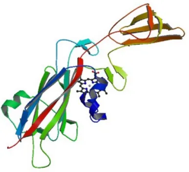
1.1 The tertiary structure of plastocianin (PDB ID: 1PLC). . . 4

1.2 The structure of plastocianin active site. The red sphere is copper ion. . . 5

1.3 The tertiary structure of cytochrome f (PDB ID: 1CTM). . . 6

1.4 The heme group of cytochrome f. . . 6

1.5 The tertiary structure of the eukaryotic 60S ribosome. . . 7

1.6 The general steps for molecular docking. . . 9

1.7 Two models of molecular docking. . . 10

1.8 The schematic of periodic boundary condition (PBC). The central cell of PBC is replicated in all direction to make infinite periodic system. . . 21

1.9 The schematic of PaCS-MD procedure. . . 26

2.1 (a) The structure of CA I in complex with the ligand, Zn²⁺, and water molecules are placed into a cubic box. CA I is represented by cartoon model. Ligand and Zn²⁺ ion are represented by VDW model and silver spheres, respectively. (b) The cluster model of CA I active site in Zn²⁺ ion which is tetrahedrally coordinated with three histidine residues (His 94, 96, 119) and ligand molecule. . . . 33

2.2 The potential energy surface (PES) (a) PES for bond distance between Zn and X (X=N(His94, His96, His94)), (b) PES for bond angle X-Zn-Y ((X,Y)= (N(His94), N(His96)), (N(His94), N(His119)), (N(His96), N(His119)) . . . 36

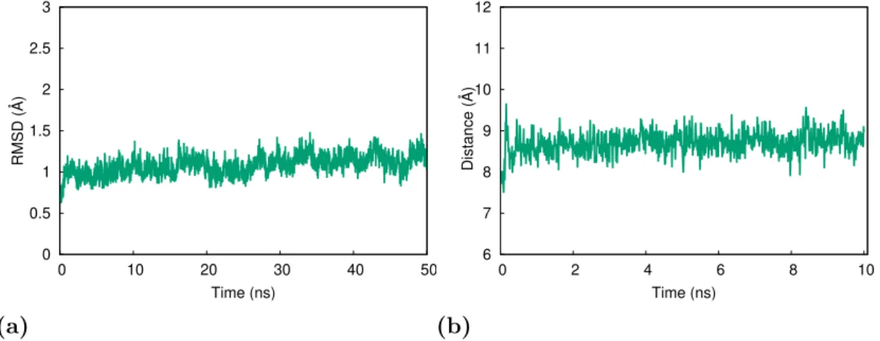
2.3 (a) The RMSD value of CA I-Ligand complex, (b) the distance between the center of mass of ligand and that of CA I enzyme during the simulation. . . 37

2.4 (a) The distance and (b) angle fluctuation in the CA I active site during the simulation. . . 38

2.5 (a) The mean force < F(r⁰) > and (b) free energy profile G(r) as a function of the distance between the center of mass of ligand and that of CA I active site. The error bars represent the standard deviation for all the trajectories of MD simulation . . . 39

2.6 The radial distribution function (RDF) of the distance between the center of mass of ligand and that of CA I active site. . . 41

2.7 The free energy profile obtained from RDF data in Figure 2.4. . . . 41

ix

(11)

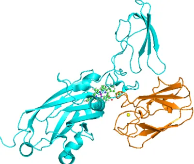
A.1 The tertiary structure of Pc-Cytf complex. Plastocianin (orange color) and cytochrome f (cyan color) are represented by cartoon models. The atom metals of iron and cupper ions are represented by magenta and yellow spheres, respectively. The heme group of Cytf is showed in stick and ball model. . . 56 A.2 (a) The cluster model of plastocianin and (b) cytochrome f in the

active site. . . 56 A.3 The snapshot structure of Pc/Cyt f complex at the distance 30 ˚A . 60 A.4 Potential energy surface (PES) for bond distance of plastocianin

active site. . . 62 A.5 Potential energy surface (PES) for angle distance of plastocianin

active site. . . 63 A.6 Potential energy surface (PES) for bond distance of cytochrome f

active site. . . 64 A.7 Potential energy surface (PES) for angle distance of cytochrome f

active site. . . 65 A.8 The RMSD value of PC/Cyt complex during the simulation . . . . 66 A.9 (a) The distance between the center of mass of plastocianin and

cytochrome f and (b) the distance between Cu ion in plastocianin and Fe ion in cytochromef for the last 2 ns. . . 66 A.10 (a) The mean force < F(r⁰) > and (b) free energy profile G(r) as

a function of the distance between the center of mass of ligand and that of CA I active site. The error bars represent the standard deviation for all trajectories of MD simulations. . . 68 A.11 The correlation between the orientation angle (θ,φ) and the mean

force < F(r⁰) > for 25 models at 3 ns MD simulations, (a) the models of complex without any constrain and (b) the other models with constraint on the distance between the center of mass of plastocianin and cytochromef atr= 30 ˚A. . . 69 A.12 The structure of plastocianin and cytochrome f represent as pur-

ple and green colors, respectively. The reference coordinates used to define the orientational and positional restrains. The spheri- cal coordinates r (P1-P1⁰ distance), θ (P1⁰-P1-P2 angle), and ψ (P1⁰- P1-P2-P3 angle), relate the position of cytochrome f respect to plastocianin. The Euler angles, Θ (P1-P1⁰-P2⁰, Φ (P1-P1⁰-P2⁰- P3⁰, and Ψ (P2-P1-P1⁰-P2⁰, determine the relative orientation of cytochrome f. . . 74 A.13 PMFs corresponding to each contribution of Table A.3 . . . 75 A.14 The standard binding free energy using a geometrical route. . . 75

(12)

B.1 (a) The structure of Model 1 is obtained from the crystal structure (PDB ID: 1TKW) and (b) Model 2 is extracted from Pc/Cytf complex, where the plastocianin has not contact with cytochromef.

These models are used to obtain the association/dissociation pathways of plastocianin in complex with cytochrome f. Plastocianin (magenta color) and cytochrome f (cyan color) are represented by cartoon models. The atom metals of cupper and iron ions are represented by green and red spheres, respectively. . . 82 B.2 The schematic of PaCS-MD procedure. . . 83 B.3 The magenta line represents the distance between center of mass

position of Pc/Cytf complex and cyan line represents the distance between metals of iron and cupper ions corresponding to model 1 to describe the dissociation pathway of plastocianin in complex with cytochrome f. (a) Those of reactive trajectories are obtained by PaCS-MD simulations, (b) those of trajectories are obtained by 10000-ps CMD. . . 86 B.4 The magenta line represents the distance between center of mass

position of Pc/Cytf complex and cyan line represents the distance between metals of iron and cupper ions corresponding to model 2 to describe the association pathway of plastocianin in complex with cytochrome f. (a) Those of reactive trajectories are obtained by PaCS-MD simulations, (b) those of trajectories are obtained by 10000-ps CMD. . . 87 B.5 The topology picture of PaCS-MD simulation from 10 multiple in-

dependent molecular dynamics (MIMD) correspond to number of cycle. (a) Dissociation pathways in model 1 and (b) Association pathways in model 2. The reactive trajectories are marked by red lines. . . 88 B.6 The free energy landscape as a function of the distance between cen-

ter of mass position of Pc/Cytf complex for model 1. In total, 300 ns-MD of simulation time is used to perform multiple independent umbrella sampling (MIUS). . . 89 B.7 (a) Model 3 and (b) Model 4. Blue and red colors represent the

structure of plastocianin and cytochrome f, respectively. Model 3 is interacted PC-Cytf complex obtained from the crystal structure, and model 4 is an independent model where the distance between the protein is more than the cutoff. . . 91 B.8 MSD of Model 3 . . . 92

(13)

(14)

1.1 The several softwares are used for molecular docking. . . 11

2.1 Bond and angle parameters of zinc ion in the CA I active site. The standard deviations are shown in parentheses. . . 37

2.2 The binding free energy and the contribution of each energy term. The standard deviations are shown in parentheses. Units are in kcal/mol. . . 42

A.1 Bond and angle parameters of plastocianin active site. . . 62

A.2 Bond and angle parameters of cytochrome f active site. . . 64

A.3 The standard binding free energy using a geometrical route.. . . 76

xiii

(15)

(16)

General Introduction

1.1 Overview of the Thesis

This doctoral thesis is a summary of my research concern in the theoretical studies on the binding free energy, association/dissociation pathways and free energy landscape by all-atom molecular dynamics simulation (MD), parallel cascade molecular dynamics (PaCS-MD), and molecular docking simulations. For the investigation of ligand-receptor complex, we have selected the complex of carbonic anhydrase (CA) I with ligand molecule. We have estimated the free energy profile of ligand dissociation in the CA I enzyme by performing all-atom MD simulation combined with thermodynamic integration method. For the protein-protein complex, we have investigated the binding free energy of plastocianin and cytochrome f complex by MD simulation. Association/dissociation pathways of protein complex are estimated by performing PaCS-MD. The outlines of my research topics at Gradu- ated School of Natural Science and Technology, Kanazawa University during PhD study are presented by following steps:

Molecular Dynamics Study of Free Energy Profile for Dis- sociation of Ligand from CA I Active Site

We have investigated the dissociation process of ligand molecule form the carbonic anhydrase (CA) I by using all-atom MD simulation combined with thermodynamic integration. The structure of CA I active site contains the zinc. Thus, the force

1

(17)

field parameters of zinc ion are estimated by quantum chemical calculation. We discussed the binding free energy as a function of the distance between the center of mass position of CA I active site and ligand molecule. We also discussed some thermodynamic properties such as the binding free energy, the equilibrium state of the free energy surface and so on.

M.S. Arwansyah, Koichi Kodama, Isman Kurniawan, Tatsuki Kataoka, Kazu- tomo Kawaguchi and Hidemi Nagao. Molecular dynamics study of free energy profile for dissociation of ligand from CA I active site. Science Report Kanazawa University, 63, pp. 15-28, 2019 (Published).

Theoretical Study of the Binding Free Energy of Plasto- cianin and Cytochrome f complex

We have investigated the binding free energy of plastocianin and cytochrome f complex by using all-atom MD simulation. The force field parameters in the active site of plastocianin and cytochrome f were calculated by quantum chemical calculation. We discussed the free energy profile as a function of the distance corresponding to the dissociation process of the plastocianin in complex with cytochrome f. We also discussed the viewpoint of the dependency of the angle structure and properties in the protein complex and has been summarized in the this letter.

M.S. Arwansyah, Kazutomo Kawaguchi and Hidemi Nagao. Theoretical Study of The binding Free Energy of Plastocianin and Cytochrome f complex. Science Report Kanazawa University, 2020 (In prep.).

Theoretical Study of Association/Dissociation Pathways of Plastocianin and Cytochrome f Complex by Parallel Cas- cade Molecular Dynamics Simulation

We have investigated the association/dissociation pathways of plastocianin and cytochrome f complex by using parallel cascade molecular dynamics (PaCS-MD) Simulation. The selected reactive trajectories during the simulation are used to perform the next cycle until obtain the association/dissociation steps along the

(18)

simulation. To validate the stable state of the Pc-Cytf complex in dissociation pathway, we calculate the free energy landscape by using multiple independent umbrella sampling (MIUS). The initial configuration obtained from PDB file is used to provide the distance constraints. From our simulation, we obtain the flat energy landscape at the distances 37 to 44 ˚A. This flat energy is crucial part for determining the conformation of the Pc-Cytf complex in relation to the dissociation process.

M.S. Arwansyah, Kazutomo Kawaguchi and Hidemi Nagao. Theoretical Study of Association/Dissociation Pathways of Plastocianin and Cytochrome f complex by PaCS-MD Simulation. International Journal of Modern Physics C, 2020 (In prep.).

1.2 Introduction to Plastocianin and Cytochrome f

In photosynthesis process, the plant or other organism convert light energy into the various chemical reactions that result the energy for the organism activities.

This energy is placed in carbohydrate molecules which are produced from carbon dioxide and water molecule. In plant, the thylakoid lumen of chlorophyll, which is found in chloroplast, contains structures within the membranes called photosys- tems one and two and also in this lumen contains the proteins to adsorb light energy and donate the excited electrons to carriers in an electron transport process.

Some proteins consisting of plastoquinon, cytochrome, plastocyanin, ferredoxin and NADP reductase are used as carriers for transport one electron to another in a series of redox reaction [1–3]. The series of the electron transfer mechanism are found in thylakoid membrane of chlorophyll.

In photosystem II, an electron which is released from the chloropyll molecule with a higher energy level easily moves from the chlorophyll to the electron acceptor molecules. Water molecules replenish the lost electrons and dissociate the hydrogen ions and release the oxygen gas. Meanwhile, the electrons as the exicited electron continue the along electron transport chain and reduce the plastoquinon.

The electrons move from the plastoquinon in oxidized state to cytochrome which becomes the reduced cytochrome. Then, the reduced cytochrome passes electrons to plastocianin. From plastocianin, the electrons are replenished since in the

(19)

Figure 1.1: The tertiary structure of plastocianin (PDB ID: 1PLC).

photosystem I, the excited electrons obtained from chloropyll are used to reduce ferredoxin. NADP reductase uses the excited electrons and protons from stroma to reduce NADP⁺ producing NADPH and hydrogen. This NADPH is later used to fuel the energy consuming sugar production of photosynthesis [1,4–6].

In thylakoid membrane, some proteins including plastocianin and cytochrome are used for electron transport in a series of redox reaction. Plastocianin has a function to catches one electron from cytochromef in cytochrome b6f complex (photosystem II) to chlorophyll (photosystem I). Plastocianin is one of the copper protein which contain one copper ion in the active site [7, 8]. Plastocianin is grouped as type I copper is known as one of the blue copper protein or cupredoxin. Three group of copper protein can be classified based on their properties and magnetic measurement, i.e type I copper (T1Cu), type 2 copper (T2Cu), and type 3 copper (T3Cu) [9].

Plastocianin contains 99 residues which consist of a copper ion, eight strands of beta-sheet, two helix structures and connected with seven turn structures. The total number of atom of plastocianin is 1548 atoms. The structure of plastocianin is shown in Figure 1.1. The active site of plastocianin consists of the copper ion coordinated in a trigonal planar structure with two nitrogen atoms of the imidazole group of histidine, i.e. His-37 and His-87, one sulfur atom of cystein (Cys-84), and also one sulfur atom of methionine (Met-92) is bound to the copper ion as axial ligand [7,9]. The structure of active site of plastocianin is provided in Figure 1.2.

(20)

Figure 1.2: The structure of plastocianin active site. The red sphere is copper ion.

Cytochrome f is a protein subunit found in the tylakoid membrane of chloroplast which has crucial function for the electron transport in the scheme of photosynthesis. In a series of redox reaction, this protein involves as an acceptor of the electron then transport the electron to the plastocianin. Cytochrome f is the largest of the four polypeptide in cytochrome f b₆f. This polypeptide is classified as a c-type cytochrome where the spectroscopic studies shown the value of ab- sorption maximum at th 554 nm and a midpoint oxidation potential of -365 mV at pH 7. Cytochrome f contains 250 residues which consist of a heme compound and two soluble structure domains in the lumen-side segment [10]. In the intact cytochrome, 250 residues associate the extrinsic domain to the membrane anchor helix. The structure of cytochrome f can be seen in Figure 1.3.

The crystal structure of cytochrome f has been investigated by X-ray analysis [11]. Cytochrome f has the unique fingerprint sequence, i.e. Cys-X-Y-Cys-His, of c-type cytochrome which is important to make the covalent bond of heme group.

The heme compound is composed by iron atom bound to a porphyrin acting as a tetrahedral ligand, and one or two axial ligands [10, 11]. The heme group of cythocrome f was presented in Figure 1.4.

(21)

Figure 1.3: The tertiary structure of cytochrome f (PDB ID: 1CTM).

Figure 1.4: The heme group of cytochrome f.

1.3 Introduction to 60S Ribosomal Subunit

Ribosome is a complex macromolecule containing variety of ribosomal proteins and ribonucleic acid (RNA) which catalyze the protein synthesis in cell [12, 13].

This molecule consists of two subunits, a large (80S) and a small (70S) subunit, with different functions [14,15]. In eukaryotic, the sedimentation at 80S ribosome is obtained with the counterparts of 40S and 60S subunits, while the counterparts of 30S and 50S subunit of 70S ribosome are found in prokaryotic. The catalytic sites of the peptidyl transferase center (PTC) catalyze the bond formation and hydrolyze the peptidyl-tRNA during the protein synthesis. These biological mechanisms are worked in the large ribosomal subunit. The small subunit has the

(22)

Figure 1.5: The tertiary structure of the eukaryotic 60S ribosome.

sequence of codons on mRNA in relation to the decoding site for the synthesis of a polypeptide chain [16–18].

In the last decade, the scientific work on the investigation of the prokaryotic translation mechanism has increased by showing the number of publication of the crystal structure of the small (30S) and large (50S) subunit ribosomal subunit. In atomic resolution, the structures of prokaryotic ribosome in binding with protein factors in relation to the translation process have showed us the various stage of protein synthesis with molecular snapshot structure [14,19,20]. However, the understanding of the molecular synthesis in eukaryotes needs more investigation because the protein synthesis mechanism remains less information.

Eukaryotic ribosome is significantly larger than that of the prokaryotic counterparts because the numerous RNA extension segments growed with specific ribosomal protein molecules. Therefore, the eukaryotic 60S subunit in yeast (T.

thermophilia) is larger than 50S subunit in prokaryotic (Eschericia coli) with the values of 2 million daltons and 1,3 million daltons, respectively [21]. Because of the structural complexity of the eukaryotic ribosome, it affects the functional differences between prokaryotic and eukaryotic. In eukaryotic cells, the ribosome biogenesis is complicated which involves 200 trans-acting protein on the process- ing and modification mechanism of RNA, bring in the ribosomal proteins into the nucleus and transport to the preribosomal into the cytoplasm [16].

(23)

Recently, the 60S ribosomal subunit is issued to understand the several regulatory during the initiation process. The crystallography structure of the T. thermophilia 60S ribosome subunit as shown in Figure 1.2 was solved by Klinge and co-workers [21]. This molecule contains three rRNA molecules, i.e. 5S, 5.8S and 26S rRNA where the 5.8S rRNA placed the same region as the 5’ end of the prokariotic 23S rRNA. Two clusters of RNA counterpart operate as the binding mode for eukaryotic-specific proteins [22, 23].

The structure of the 60S ribosome contains 42 proteins, where 20 proteins are allocated between eukarya and archea, 16 proteins exist in all domain of life, and only 6 proteins are eukaryotic-specific parts [21]. The critical for creating an intricate protein-RNA network is involved in the ribosomal proteins which contain the eukaryotic-specific extension. Some of these regions are found as core area for the active site and the exit tunnel. The 26S rRNA is the important region of ribosome because the peptidyl transferase center, the exit tunnel and antibiotic binding sites can be found at this domain. 26S rRNA contains all area essential for catalysis and subtrate binding, i.e. A, P, and E-sites. Therefore, both prokaryotic and eukaryotic ribosome at 26S rRNA region become an interesting targets for amount of the antibiotics [24, 25].

1.4 Introduction to Molecular Docking

Molecular docking is a method to predict the binding affinity between receptors and ligands and estimate the stability of the complex. Docking is a good technique to estimates the binding orientation of drug candidate (ligand) against the target molecule in order to understand the activity of the drug. Thus, this method is useful technique for the drug design and process. In recent years, the crystal structures of protein have been significantly investigated and have been provided in a database such PDB database. With an increasing of the database of the crystal structure, molecular docking is widely used by researchers to know the molecular interaction of ligand-protein complex in relation to improve the drug target predictive capacity [26–29]. Furthermore, this method greatly uses to reduce the research cost. The steps for molecular docking are summarized in Figure 1.6.

(24)

Figure 1.6: The general steps for molecular docking.

In molecular docking, two stages are applied to understand the molecular mecha- nisme: docking the ligand into the receptor molecule (pose identification) and pre- dicting the docked conformation value binding to the target molecules (scoring).

The accurate algorithms are created to obtain the better prediction capacity of the complex by concern on the conformation and orientation of the small molecule in the active site of target molecule and also the algorithm evaluates the molecular interaction by providing the scoring function of the binding affinity. The various algorithm for docking analysis, i.e, Genetic algorithm, Monte Carlo, Systematich Searches, Distance Geometry, Fragment-Based, and etc. are commonly used to determine the binding modes [30, 31].

In order to evaluate and rank the predicted ligand conformation into the molecule target in the structure-based virtual screening, the scoring function is a good approach to find the best binding affinity of the complex because the best scoring ligands are the best binders. Scoring function are classified into the three class:

knowledge-based, force field, and empirical [31]. Knowledge-based scoring function is used to observe the similarity attribute of the known coordinates obtained from experimental structure of a large set of protein-ligand complex. The attributes such atom-atom distances between the complex are contributed to estimate the binding affinity after converting a pseudo-energy function of pairs of atoms in the protein-ligand complex. The force field scoring functions is based on the molecular mechanic force filed where the potential energy of a complex is obtained from the bonded and non-bonded interactions. The binding affinity of the ligand-protein

(25)

Figure 1.7: Two models of molecular docking.

complex is expressed by the estimation of the van der Waals energy and electrostatic energy terms where these energy terms are presented by a Lennard-Jones potential function and Coulumbic potential function. Lastly, empirical scoring function is based on the several parameters such as the hydrogen bonding, van der Wall interactions, hyrophobic interactions and the ligand’s conformational entro- phy which are utilized to estimate the binding affinity [32–34].

In molecular docking, two models represent the action of ligand to the target molecule which refer to the lock-and-key model and induced fit model [35]. The lock-and-key model denotes to the rigid docking of receptors and ligand to obtain the proper orientation for the key to the open up the lock. The geometric complementarity is crucial for this model. Meanwhile, the induced fit model is established by some parameters including geometrical and energy complementarity and pre- organization which promise that ligand and the target molecule find the stable complex by the conformation of the complex is modified to fit each other in the binding pocket. This docking process is known as flexible docking. The scheme for two model of molecular docking is described in Figure 1.7. The several docking programs are commonly used to perform molecular docking shown in Table 1.1.

(26)

Table 1.1: The several softwares are used for molecular docking.

Name Search algorithm Scoring function Feature

AutoDock Vina GA (genetic algorithm) Semi empirical calculation Flexible-rigid docking

FREED Shape fitting (gausssian) Screen score Flexible docking

Glide Exhaustive systematic search Semi empirical calculation Flexible docking AutoDock GA (genetic algorithm) Semi empirical calculation Flexible-rigid docking Gold GA (genetic algorithm) Semi empirical calculation Flexible docking ZDOCK Geometric complementarity and MD Molecular force field rigid docking

1.5 Introduction to Molecular Dynamics Simu- lation

Molecular dynamics (MD) is a method to obtain the information of the time evolution of atom or molecule in relation to obtain the thermodynamic properties computed according to Newton’s second law. MD method is widely used to calculate the large number of particles such as protein or other biological macromolecules. This method can be utilized to quantity the properties of a system where the macroscopic quantities are extracted from the microscopic trajectories of molecules. Therefore, the characteristic of atom/molecule can be used to represent the macroscopic of physics properties. MD has many purposes to find the structure and dynamics of macromolecules, thermodynamics properties of gas, liquid, and solid, transport phenomena, and etc [36, 37] .

MD method has been applied since 1950s where Alder and Wainwright conducted the earliest MD simulation on the hard-sphere model. Real atomic interactions are applied on continuous potential [38]. In 1976, the first simulation on protein was performed because computational tools became more widespread [39]. The empirical energy function is developed based on the physics-first principle assumptions.

The initial protein MD simulation, short time simulation around 9.2 ps has been perform on the small bovine pancreatic trypsin inhibitor (BPTI). Since 1998, a longer simulation time of ten nanoseconds was implemented [40]. Now, the modern theory and algorithm of MD method has been utilized to consider more the realistic model on the system by immersing water molecules, ions, and etc. In this section, we represent the brief MD simulation concepts such as the mathematical solution of the differential equation from Newton’s formula, The common force field, boundary condition, MD system with NVT and NPT ensembles and etc.

(27)

1.5.1 Integration Outline

Molecular dynamics use some algorithms by solving differential equation from Newton’s formula. Some integration approaches are discussed and summarized by following subsections.

1.5.1.1 Verlet Algorithm

Verlet algorithm is particularly suited for MD simulation. This algorithm has been widely utilized in many aspects on molecular simulation for liquid and solids to biological molecules. The schematic integration is written as follows:

F_i =m_id²ri

dt² , (1.1)

whereF_i is the total force acting on thei-th particle,m_i is the mass of the particle i, and r_i is the position vector of the particle. To get approximate difference formula for derivatives, Taylor expansion for position around time (t) is expressed by following equation:

r(t+ht) = r(t) +v(t)ht+1

2a(t)ht²+b(t)ht³+Oht⁴ (1.2) The time is reversed and we find a function:

r(t−ht) = r(t)−v(t)ht+1

2a(t)ht²−b(t)ht³+Oht⁴ (1.3) then, we combine equation 1.2 and 1.3, we get an approximation for the first derivative,

r(t+ht) = 2r(t)−r(t−ht) +a(t)ht² +Oht⁴ (1.4) The function is update equations for position. It is similar for velocity update by following equation:

v(t) = r(t+ht)−(t−ht)/2ht (1.5)

(28)

In Verlet algorithm, equation 1.4 and 1.5 are the update equations. The position and acceleration at time t and position at previous time step as input are used for Verlet algorithm.

r(t₀−ht) = r(t₀)−v(t₀)ht (1.6) Forward time step equation

r(t+ht) = 2r(t)−r(t−ht) + 1

mF(t)ht² (1.7)

Reverse time step (replace ht with -ht)

r(t+ (−ht)) = 2r(t)−r(t−(−ht)) + 1

mF(t)(−ht)² (1.8)

r(t−ht) = 2r(t)−r(t+ht) + 1

mF(t)ht² (1.9)

From equations above, we have similar algorithm to shift system backward with similar force and position. Verlet algorithm accurately estimates the position and velocities in order of ht² and ht⁴, respectively.

1.5.1.2 Leap-Frog Algorithm

Leap-Frog algorithm can be found by simple mathematics calculation of the Verlet integrator. This algorithm excludes one of the component of Verlet algorithm, i.e., small numbers Oht² to differences in large ones O ht⁰. In this diagram, first velocity at half time step is estimated for updating the position at full time step.

The equation for leap-frog algorithm is provided as follows:

r(t+ht) =r(t) +v(t+ 1

2ht)ht (1.10)

v(t+ht) =v(t− 1

2ht) + 1

mF(t)ht (1.11)

Substituting equation 1.9 in equation 1.10 to obtain the equivalent algorithm between Leap-Frog and Verlet.

(29)

r(t+ht) =r(t) +

v(t− 1

2ht) + 1

mF(t)ht

ht (1.12)

From the equation 1.9, we can also obtainr(t) estimated at previous time step as following equation:

r(t+ht) = r(t−ht) +v(t− 1

2ht)ht (1.13)

Substitutingv(t−¹₂ht) from above equation into the equation 1.10, and we obtain

r(t+ht) =r(t) +

(r(t)−r(t−ht)) + 1

mF(t)ht²

,

= 2r(t)−r(t−ht) + 1

mF(t)ht²

(1.14)

Equation 1.13 is equivalent to the original Verlet presented by equation 1.4. In Leap-Frog algorithm, it is need to have velocity at the previous time step which can be obtained by simple approximation:

v(t₀−ht) = v(t₀)− 1

mF(t₀)1

2ht (1.15)

The velocity at current step can be obtained by using a simple interpolation as following equation:

v(t₀−ht) =

v(t+ 1

2ht) +v(t−1 2ht))

(1.16) The advantage of the Leap-Frog integrator is no need to add number that are different order in ht.

1.5.1.3 Velocity-Verlet Algorithm

In the position Verlet and Leap-Frog integration, the velocity is discussed accurately. Another approach to handle the velocity properties is presented by Velocity-Verlet algorithm (Verlet scheme) as following equation:

(30)

r(t+ht) = r(t) +v(t)ht+ 1

2mF(t)ht² (1.17)

v(t+ht) =v(t) + 1

2m[F(t) +F(t+ht)]ht (1.18) From these equations, we can obtain the Verlet algorithm by eliminating the velocity. This algorithm needs the position, velocity, and acceleration at current time step. Also, it involves one intermediate step. Updating the first position with equation 1.4, then the velocities at mid step are handled by using

v(t+ 1

2ht) =v(t) + 1

2m[F(t)]ht (1.19)

The force and acceleration at time t+ht are handled and velocity is computed as follows:

v(t+ht) = v(t+ 1

2ht) + 1

2m[F(t+ht)]ht (1.20) This equation is the most preferred as integrator due to stability, accuracy and simplicity.

1.5.1.4 Higher order integrator

A better accuracy both in position and velocity becomes crucial part to select the integrator. Higher order scheme can be applied where the scheme allows to use larger time step without compromising on energy accuracy. But, this scheme is not time reversible and do not have a preserving part. The main idea for predictor- corrector algorithm is provided as follows:

1. Predictor: The position and its derivatives at timet, i.e., velocity, acceleration, and etc, are used to find the position and its first derivatives at time t+ht.

2. Force assessment: The predicted position is applied to handle the force and acceleration at the predicted positions.

3. Corrector: The new acceleration is used to correct the predicted position, velocity and acceleration.

(31)

Taylor expansion is applied at the position at time t+ht

r(t+ht) = r(t) +v(t)ht+ 1

2a(t) + 1

6b(t) + 1

42c(t) +... (1.21) Where v is the velocity, a is the acceleration, b is the third derivative of the position, and cis the fourth derivatives etc.

By using Taylor expansion for velocity, acceleration and etc, the equations become as follows:

v(t+ht) = v(t) +a(t)ht+ ht²

2 b(t) + ht³

6 c(t) +... (1.22)

a(t+ht) = a(t) +b(t)ht+ ht²

2 c(t) +... (1.23)

b(t+ht) = b(t) +c(t)ht+... (1.24) The predicted (step 1) and calculated (step 2) acceleration are computed by following equation:

∆(t+ht) = a^c(t+ht)−a(t+ht) (1.25) This equation is used to improve the position and velocity in the correction step as following equations:

r^c(t+ht) = r(t+ht) +c₀∆a(t+ht) (1.26)

v^c(t+ht) = v(t+ht) +c₁∆a(t+ht) (1.27)

a^c(t+ht) = a(t+ht) +c2∆a(t+ht) (1.28)

b^c(t+ht) = b(t+ht) +c₃∆a(t+ht) (1.29)

(32)

The value of the coefficients depends on the order given by Taylor expansion.

1.5.2 Analysis on Force fields

The empirical forms and the total potential energy are described by the inter and intra-molecular represented by following equation:

E_total =E_vdW +E_elec+E_bond+E_angle+E_torsion (1.30) Where E_total =E_vdW +E_elec+E_bond+E_angle+E_torsion are the total energy, van der Waals, electrostatic, bond stretching, angle bending, and torsion energy con- tributions, respectively.

The 12-6 LJ interaction is used to represent the van der Waals interaction given by

E_vdW =D₀ (

R0

R 12

−2 R0

R 6)

(1.31)

WhereD₀ is the strength of the interaction andR₀ is the range of interaction. The constant can be obtained by quantum calculation of by experimental value. 12-6 LJ interaction parameters are provided by atom types from general force fields obtained in AMBER, CHARMM, and etc. Other form of non-bond interaction is also generated by Buckingham potential given by

EBuckingham = X

nonbonded pair

Aexp(−crik− B r⁶_ik)

(1.32)

In this constant value of these potential are provided in available force fields. To handle the special coordination using non-bond interaction, Morse potential can be applied and the equation is provided by

E_{M orse} = X

nonbonded pair

D₀

1−e^−α(R−R⁰⁾ 2

(1.33) Where D₀,R₀, and α are constants.

(33)

Coulomb’s law given in equation 1.32 are used to represent the electrostatic interaction between charges particles.

E_Coulumb = X

nonbonded pair

q_iq_k

r_ik (1.34)

q_i and are charge on each atom and dielectric constant, respectively. This interaction is computational cost due to its long range character

The bond stretching potential can be presented by the harmonic potential. This potential is used to describe the intra-molecular interaction.

E_bond(r_ij) = 1

2K_b(r_ij −r₀)² (1.35) Other potential to describe the intra-molecular interaction is provided by Morse potential. This is particularly useful for handling specific coordination in a given geometry.

E_{M orse} = X

1,2pairs

D_b

1−exp[exp−K_m(r−r₀)] (1.36)

Where D_b and K_m represent the well depth and well width, respectively.

The angle bending potential is also described by the harmonic potential form given by:

E_angle(θ_ijk) = 1

2K_θ(θ_ijk−θ₀)² (1.37) In case of cosine harmonic theta, the angle bending potential is provided by

E_angle(θ_ijk) = 1

2K_θ(Cosθ_ijk−Cosθ₀)² (1.38) To handle certain structure of molecular system as a part of bond stretching and angle bending, the torsional potentials are included. Two type of this potential, i.e.

dihedral angle and improper torsion. To constrain the rotation around the bond, the dihedral angle is commonly applied. This potential is involved four consecutive bonded atoms (i-j-k-l). Meanwhile, improper torsion is used to handle planarity

(34)

of certain atoms where four atoms are not bonded in the same sequence as i-jk-l.

One of the commonly applied dihedral potential is the cosine form provided by E_(φ_ijkl) =X

n

V_n

2 [1 +cos(n)φ_ijkl−φ₀] (1.39)

Where n is an integer. φ and n represent the rotational sequence and the period- icity of the rotational barrier, respectively. V_n and φ₀ are the associated barrier height and reference torsion angle.

Commonly applied improper torsion is harmonic form and is represented by following function:

E_(ϕ_ijkl) = k^I_1,j,k,l(ϕ_ijkl−ϕ₀)² (1.40) Where k_1,j,k,l^I is the force constant.

1.5.3 Application of SHAKE Algorithm

In this case, the optimum choice of the integration time step for numerically stable integrator as well as better energy conservation is presented. In molecular system, the selected of time step is restricted by the various time scales related with degrees of freedom such as bond vibration, angle stretching, and torsional form. The wave number and time scale in respect to vibrational mode of O-H, N-H stretch are 3200-3600 cm¹ and 3,1 fs, respectively. For H-O-H (1600 cm¹) bend and O-C-O (700 cm¹) have time step 6.5 fs and 15 fs, respectively. Therefore, the system containing hydrogen bond is suggested to use 1 fs to avoid any problem with energy conservation. Another solution, bonds involving H with highest frequency are constrained during simulation and larger time step can be applied. Ryckaert and co-workers introduces SHAKE algorithm to constrain bond with hydrogen atom [41]. This algorithm is widely used in molecular simulation. The basic idea of this algorithm is to apply the Lagrange multiplier to impose bond distance constant. Assuming, we have N_c such a constraint provided by

α_k =r²_k₁_k₂ −R²_k₁_k₂ = 0, wherek = 1,2,3...N_c (1.41)

(35)

R_k²

1k2 is constrained distance between atoms k_i and k₂. From this equation, it is modified constraint given by

m_id²r_i

dt² =f rachh_r_i[V(r_i...r_N) +

Nc

X

k=1

λ_k(t)α_k(r1....r_N) (1.42)

Where m_i is mass of i ^th particle and λ_k is the Lagrange multiplier for k^th constraint. This equation can be answered for unknown multiplier by solving N_c quadratic coupled equations. The equation of motion is given by

r_k₁(t+ht) =r_k^uc

1(t+ht) + 2(ht)²m⁻¹_k

1λ_k(t)r_k₁_k₂(t) (1.43)

r_k₂(t+ht) =r_k^uc₂(t+ht) + 2(ht)²m⁻¹_k

2λ_k(t)r_k₁_k₂(t) (1.44) Wherer^ucis the position updates with unconstrained force. This route is replicated till defined tolerance τ given as

[r_k₁_k₂(t+ht)−R_k1k2

R_k1k2 ]≤τ (1.45)

1.5.4 Periodic Boundary Condition

In molecular dynamics simulation, systems containing few thousands of atoms are simulated in the simulation box. Such small systems are dictated by surface effects-interactions of the particles with the container walls. To prevent the surface effect and to provide thermodynamics properties on the behavior of the bulk liquid, periodic boundary condition (PBC) is applied. PBC cell is repeated in all directions to make an infinite lattice as shown in Figure 1.8. Atoms/particles in the central cell are considered during simulation. Therefore, if a particle moves in the central cell, its periodic image also moves in the same direction and when a particle moves away from the central cell, its periodic images exist from the op- posite face. By this PBC, we can discuss that there is no rigid boundary wall and the number of atoms in the central simulation cell is kept during the simulation.

(36)

Figure 1.8: The schematic of periodic boundary condition (PBC). The central cell of PBC is replicated in all direction to make infinite periodic

system.

The interaction energy between atoms in the PBC cell becomes crucial important to imply the interaction phenomena along simulation. A particle (i) interacts with all other particles in infinite periodic system. We can assume that all intermolec- ular interactions are pairwise preservative and the total energy of N particles in any one periodic cell can presented as U_tot = ¹₂P

i,j,nu(| r_ij +nL |) , where L is diameter of the periodic box cell and n is an arbitrary vector of their integer numbers, the prime over the sum represents the term with i=j is to be excluded when n= 0.

1.5.5 Thermostat and Barostat

The algorithms are explained by previous discussion is appropriate for Micro canonical ensemble (NVE ensemble), where the total energy of the system is a constant of motion. In molecular system, Canonical ensembles known as NVT and NPT are commonly used to keep temperature or pressure in constant condition.

In this case, we discuss two very commonly applied route for doing simulation in canonical ensembles such as velocity rescaling method and weak coupling method of Berendsen [42].

(37)

1.5.5.1 Velocity Rescaling Method

The temperature of the system during simulation is estimated from the kinetic energy using equi-partition theorem as following equation:

E_KE = 3

2N k_BT (1.46)

The simplest manner to keep a constant T is to rescale the velocity consistent with the desired temperature. Assume at time t is T(t) and desired temperature is T_desired. The change in temperature provided in equation below can be worked when the velocities are multiplied by a factor λ.

∆T = 1 2

N

X

i=1

2 3

m_i(λv_i)² N k_BT −1

2

N

X

i=1

2 3

m_iv_i²

N k_BT (1.47)

Therefore, we have

λ=p

T_desired/T(t) (1.48)

At each time step, the velocities are multiplied by λ and T(t) is estimated from the kinetic energy (KE) at time t. The velocity rescaling method is simple and easy to used but, it does not represent any statistical ensemble.

1.5.5.2 Berendsen Weak Coupling Method

Berendsen algorithm [42] represents a weak coupling to an external heat bath to keep constant temperature during simulation. by adding a stochastic and friction term, the equation of motion is modified by

m_iv˙_i =F_i−m_iγ_iv_i+R(t) (1.49) Where, τ_i is the damping constant that decides the strength of coupling with the heat bath. This τ_i is constant equal for all particles. R(t) is a Gaussian stochastic variable calculated by

(38)

< R_i(t)R_j(t+τ)>= 2m_iγ_ikT δ(τ)δ_ij (1.50) Time dependence of the total kinetic energy is provided by

dE_k

dt = lim

∆→0

"

{

3N

X

i=1

1

2miv_i²(t+ ∆t)−

3N

X

i=1

1

2miv_i²(t)}/∆t)

#

(1.51)

WhereN is the total number of particles. From the equation 1.49, the change ∆v_i of the velocity over a time internal of t = 0. ∆t is given by difference in velocity in two time step presented by

∆vi =vi(t+ ∆t)−vi(t)

= 1 m_i

Z t+∆t t

[F_i(t⁰)−m_iγv_i(t⁰) +R_i(t⁰)]dt

(1.52)

Where R is Gaussian noise. By adding equation 1.50, we get,

3N

X

i=1

Z t+∆t t

dt⁰

Z t+∆t t

dt⁰⁰R_i(t⁰)R_i(t⁰⁰) = 6N mγkT₀∆t (1.53)

Using this relation in equation 1.51, we find

dE_k dt =

3N

X

i=1

v_iF_i+ 2γ 3N

i= 1kT₀−E_k

(1.54)

First part on the right side is equal to minus of the time derivative of potential energy and its connected to the effect of the systematic force. Thus, the coupling to the heat beat is showed by the second part. This can be associated with the time dependence of the system temperature

dT

dt = 2γ(T₀−T) (1.55)

Where the time constant for heat bath coupling τ_T is equal to 2γ⁻1. Therefore, the equation of motion can be represented by

(39)

m_iv˙_i =F_i−m_iγ_i T₀

T −1

v_i (1.56)

˙ r_i

t+∆t 2

=F_i−m_iγ_i T0

T −1

v_i (1.57)

The heat bath and subsequent temperature control obtained in in the Berendsen weak coupling scheme are reached by appropriate rescaling of the velocities by a time dependent scaling factorλduring the integration of equation of motion. The scaling factor in respect to the leap-frog integrator given by

˙ r_i

t+ ∆t

2

=λ(t) ˙r_i⁰

t+ ∆t 2

=λ(t)

˙ r_i

t+ ∆t

2

+m⁻¹_i F_i(t)∆t

(1.58)

To reach the temperature variation consistent seen in equation 1.55 the scaling factor λ can be obtained by adding by

T

t+∆t 2

=T

t− ∆t 2

+τ_T⁻¹∆t

T₀−T

t− ∆t 2

(1.59)

By using equation 1.57 and 1.58 we get λ²(t)T⁰

t+ ∆t

2

=T

t− ∆t 2

+τ_T⁻¹∆t

T₀−T

t− ∆t 2

(1.60)

Solving this for λ(t) obtains

λ(t; ∆t) =

(T(t− ^∆t₂ )

T⁰(t+^∆t₂ ) +τ_T⁻¹∆tT₀−T(t− ^∆t₂ ) T⁰(t+^∆t₂ )

)¹₂

≈ (

1 +τ_T⁻¹∆t

"

T₀

T⁰(t+ ^∆t₂ −1

#)¹₂

(1.61)

(40)

Therefore, the temperature is handled by scaling the velocity of the particle for each time step with a time dependent constant as following equation:

λ=

"

1 + ∆t τ_T

T0

T −1

!#¹₂

(1.62)

A good value ofτ_T is 0.5-1 ps when integration time step ht = 1 fs. The coupling will be weak if τ_T is large meanwile, the coupling becomes strong if τ_T is small.

This algorithm is equivalent to simple velocity rescaling method when the coupling parameter equal to integration time step (τ_T =ht).

1.5.5.3 Weak Coupling Barostat for Constant P

Coupling to a bath is achieved by adding an extra term to equation of motion for relevant variable according to previous discussion in subsection Berendsen coupling. It is similar that by adding an extra term to the equation of motion that controls pressure change, coupling to constant pressure bath can be obtained. The equation of motion for pressure can be composed by

dP

dt = P₀−P

τ_P (1.63)

The pressure is presented by

P = 2

3V (E_k− ≡) (1.64)

Where

≡=−1 2

X

i<j

r_ij.F_ij (1.65)

That equation is internal virial for pair additive potentials.

µ= [1− δt

τ_p(P −P0)]¹³ (1.66)

(41)

Figure 1.9: The schematic of PaCS-MD procedure.

1.5.6 PaCS-MD simulation

Parallel cascade molecular dynamics (PaCS-MD) simulation is one of methods to investigate the conformational transition pathway of protein in respect to the folding process and association/dissociation process. The physical parameters such as force field, ensemble, periodic boundary, and etc. used in PaCS-MD are similar with that of molecular dynamics described in previous subsections. PaCS- MD method is developed by Harada and co-authors [43]. This method has been used to find the possibility of the conformational transition pathway of folding process starting from the extended structure of chignolin protein to the native structure along simulation. The folding pathway obtained by PaCS-MD is good correspondence with the results presented in Ref. [44].

To estimate PaCS-MD simulation on Pc-Cytf complex, 100-ps MD simulation is performed from the structures obtained by preliminary MD. Ten snapshot structures are randomly selected as the initial structure for the first cycle. Ten initial

(42)

structures (M= 10 runs) formulated by 100-ps MD x M is independently simulated. In each cycle, ten multiple independents molecular dynamics (MIMD) are performed and each trajectory is saved every 1 ps. Each MIMD is analyzed to evaluate simulation runs are consistent with the behavior of folding or association/dissociation of protein. The selected run from cycle 1 is taken as the initial structure for ten MIMD in the next cycle. The initial velocities are regenerated randomly to reproduce Maxwell-Boltzmann distribution for each MIMD. The selected trajectory for each cycle as joint multiple trajectories is termed as ’reactive trajectories’ proposed by Harada and co-workers [43]. These trajectories are selected to show the expected simulation during PaCS-MD. We show schematic of PaCS-MD procedure including the reactive trajectory term presented in Figure 1.9.

(43)

(44)

Molecular Dynamics Study of Free Energy Profile for

Dissociation of Ligand from CA I Active Site

2.1 Introduction

In higher vertebrates including human, 14 different CA isozymes are found in several subcellular localizations such as CAI-III and CA VII found in cytosols, CA IV, CA IX, CA XII, and CA XIV located in membrane, CA V found in mitochondria, and CA VI secreted in saliva [45, 46]. Carbonic anhydrases (CAs) family is a ubiquitous zinc enzyme which can be isolated from archaea, prokaryotes, and eukaryotes [45]. These enzymes involve the biological fundamental roles such as catalyzes of the hydration of carbon dioxide to bicarbonate which is essential to regulate the pH levels in cells, biosynthetic reaction and electrolyte secretion in several tissues [45–48].

The structures of carbonic anhydrases by X-ray analysis [49–53] have been investigated. In the enzyme active site, this enzyme contains a zinc ion which is essential for catalytic activity. Zn ion is coordinated with three histidine residues through their imidazole nitrogen atoms. A water molecule occupies the fourth coordinated position in the active site at an acidic pH (< 7) or a hydroxyl ion at higher pH.

29

(45)

The tetrahedral coordination geometry is formed through proton-transfer reaction from water binding to the zinc ion in the CAs active site [54,55]. The position of the water molecule or hydroxyl group can be changed by inhibitor to inhibit the biological process in cells. The sulfonamide group of a heterocyclic structure can also be used in the primary application as the most potent inhibitors that bind to the zinc ion through the deprotonated nitrogen. The sulfonamide group is has activities as anticonvulsant, antiglaucoma, anticancer, and antiurolithic [48].

Some diseases such as glaucoma, diabetes, cancer, epilepsy, and etc [56] is related almost every CAs family. The several ligand molecules to inhibit CAs activity are the critical target for the therapeutics against many diseases. Therefore, understanding the interaction between ligand and CAs including Zn ion is crucial. The several computational studies on CAs have been recently performed [57–59]. The interaction of some antiepileptic drugs with CA active center has been quantum mechanically investigated to elucidate the relative orientations of CA II-inhibitor complex using a high-level calculation to understanding on the mechanism of inhibitor action [57]. All-atom molecular dynamics (MD) simulation of CA enzyme has also been carried out for CA II enzyme in complex with ligand (acetazo- lamide) to obtain a theoretical understanding of metalloprotein-inhibitor complex [58]. This paper shows the quantitative insight into the binding interaction of protein-ligand complex and represents the key role in Zn ion in the CAs active site. The theoretical studies on the standard free energy of protein-ligand binding have been investigated to understand the free energy change of the ligand molecules in the binding/dissociation process [58–62].

In this research, the binding free energy between CA I enzyme and the ligand molecule is investigated. The force field parameters of the zinc ion in the CA I active site is estimated by quantum chemical calculations. The thermodynamic integration combined with all-atom MD simulation is used to calculate the free energy profile for binding/dissociation process of ligand from CA I active site according to the procedure provided in the previous work [63, 64]. We discuss the binding/dissociation process of ligand molecule by calculating the free energy profile to know the docking model of ligand into the active site of CA I related to some thermodynamic properties such as the binding free energy, the equilibrium state of the free energy surface and so on.

(46)

2.2 Method and model

In this section, we present a model using in this simulation conditions for MD simulation. The force field parameters in the CA I active site are estimated, and the free energy profile is introduced. The free energy profile as a function of the distance between the center of mass positions of CA I active site and the ligand molecule, r_cm, is calculated by all-atom MD simulation with the thermodynamic integration method presented in the previous work [62,65].

2.2.1 Model for molecular dynamics simulation

In this study, the structure of CA I in complex with the ligand molecule (4- carboxyethyl benzene-sulfonamide ethyl ester) is obtained from the X-ray crystal- lographic structure in the protein data bank solved by Srivastava,et al. (PDB ID:

2NN7) and is applied to initial structure for the simulation of ligand binding/dissociation process [66]. In the CA I enzyme, the total number of residues is 260 which consists of a zinc ion, 10 helices and 18 strands of the beta sheet with the total number of atoms being 2029. The ligand is a derivative of benzenesulfon- amide CA inhibitor which contains 17 atoms. The structure of CA I enzyme and ligand immersed by water molecules are shown in Fig. 2.1(a).

2.2.2 Force field parameters in metal

The cluster model of CA I active site consists of a zinc ion and three histidine residues (His 94, 96, 119) which are tetrahedrally coordinated with a ligand molecule as shown in Fig. 2.1(b). The CA I active site in complex with ligand is calculated by the quantum chemical methods to know the interaction effect of the stability from the interaction of zinc ion with histidine residues and ligand molecule.

The force field parameters of zinc ion in the CA I active site are not available in the Zinc AMBER force field (ZAFF) database developed by Peters et al [67].

Therefore, we evaluate the force field parameters of zinc ion in the CA I active site by calculating the potential energy surface (PES) as a function of bond distance and bond angle. The bond distance and angle potential are provided as follows:

(47)

V(r, Kr) = Kr(r−rc)², (2.1)

V(θ, Kθ) = Kθ(θ−θc)², (2.2) where Kr and Kθ are the force constants of distance and angle respectively, and rc and θc are equilibrium distance and angle, respectively. The structure of CA I is optimized by freezing the heavy atoms. The potential energy surface of bond distance and bond angle of CA I is analyzed by using the B3LYP method with the 6-31G* basis set with the increment of 0.02 and 2^◦, respectively. The range of increment is determined to avoid the inharmonic effect of distance and angle according to the suggestion in Ref. [68,69]. The optimized structure and potential energy surface calculations for distance and angle are performed by Gaussian 09 packages [70]. Then, we convert the quantum chemical calculation of the distance and angle of zinc-N(His 94, 96, 119) motif in the CA I active site into the Amber force field parameters by using Metal Center Parameter Builder (MCPB) [71].

Our force field parameters have not been submitted to the AMBER parameter database.

2.2.3 Simulation condition

All-atom molecular dynamics simulation is performed on CA I enzyme and ligand molecule. The TIP3P water model [72] with 9808 water molecules inserted in a 70× 69 ×77 ˚A³ periodic box then, 3 Cl^– ions are added to neutralize the whole system. The total number of atoms in the system is 33,425. The AMBER14 force field is used for the protein molecule [73], and general AMBER force field (GAFF) is applied to determine the force field parameters of ligand molecule. The electrostatic interactions are computed by using the Particle Mesh Ewald (PME) algorithm. The switching cutoff distance is 10 ˚A. The SHAKE algorithm is used to constrain the bond distance of the hydrogen atoms. A time step of 2 fs is applied in all simulations.

The energy minimization of the system is carried out with the constraint on the position of the heavy atoms of CA I, ligand and Cl^– ion. Then, we perform the energy minimization without any constraint. The system is simulated on N V T- constant simulation for 60 ps where the temperature is gradually increased from