Simulation of Triple Line Dynamics by Interface-Fluid Coupling

(1)

Interface‑Fluid Coupling

著者ヌルショフィアナ

著者別表示 Nur Shofianah journal or

publication title

博士論文本文Full 学位授与番号 13301甲第4146号

学位名博士（理学）

学位授与年月日 2014‑09‑26

URL http://hdl.handle.net/2297/40538

Creative Commons : 表示 ‑ 非営利 ‑ 改変禁止 http://creativecommons.org/licenses/by‑nc‑nd/3.0/deed.ja

(2)

by Interface-Fluid Coupling

NUR SHOFIANAH September 30, 2014

(3)

(4)

Ibu Masyhudah and Bapak M. Muchibbin, for their amazing love, pure sincerity, endless support and encouragement, and for everything that I can not describe it in words.

iii

(5)

(6)

In the name of Allah, the Most Merciful, the Most Compassionate. All praise be to Allah, the Lord of the worlds. I would not be able to finish my study without His amazing help. Prayers and peace be upon Mohammad, His servant and messenger.

In this opprtunity, I would like to thank my supervisor, professor Karel Svadlenka for endless support and valuable advice in both academic matter and practical life during my study. I can learn many things in my new research field, and also I can learn from him, how to be a good supervisor for my students in the future.

I would like to thank the Committe, professor Karel Svadlenka, professor Seiro Omata, professor Masato Kimura, professor Hiroshi Ohtsuka, and professor Katsuyoshi Ohara, for valuable suggestions in my dissertation.

I would like to thank the Directorate General of Higher Education (DIKTI), Ministry of National Education, Indonesia for the generous scholarship that made my study in Kanazawa University possible. And also for University of Brawijaya, especially Department of Mathematics, Faculty of Mathematics and Natural Sciences, for the approval and support for my study.

I would like to thank all of my Teachers for their great effort and sincerity since I was child and did not know everything until I can be myself now.

May Allah give more reward for all of you.

My thanks also to my labmate, Rhudaina Z. Mohammad who help me checking the grammar and many things. She is the creator of the BMO program and numerical example of interface in Section 4.1. Also thanks to all my friends that I can not mention one by one, for all the supports.

Finally, I would like to thank my beloved parents and my beloved family.

Your endless support and doa gave big influence for me. May Allah give us rahmah until together in Jannah.

v

(7)

(8)

The dissertation develops a coupled interface-network and fluid model which can serve as a first step to simulate triple line dynamics. The main ingredients of this coupled model are the interface model with nonsymmetric junctions and the fluid model in moving domain. We build an interface model based on the gradient flow of surface energy and develop a method for its numerical solution by generalizing the reference vectors and diffusion system in vector-valued BMO algorithm. Moreover, we improve the scheme by using vector-valued projection triangle and use a vector type DMF to handle volume constraint via penalization. For the fluid part, we implement a numerical method adopting DSD/SST-SUPS, a stabilized space-time finite element method in moving domain. We also apply the appropriate boundary condition which is related to a moving triple line. We couple these two models weakly via pressure acting from the fluids on the interfaces and by the fact that the interfaces determine the domain for fluid motion. In the end, we present results of numerical experiments.

vii

(9)

(10)

List of Figures

1.1 Experimental results taken from [48]: Air bubble formation in case blowing of air from a small hole in the bottom of a container filled with water with (a) stainless steel surface

(wetting) (b) waxed surface (less wetting) . . . 2

2.1 Physical setting . . . 5

2.2 Triple Junction . . . 8

2.3 Relating surface tensions to junction angles. . . 10

2.4 Physical setting . . . 11

2.5 Vicinity of triple line . . . 12

3.1 Configuration of a stable junction. . . 16

3.2 Configuration of the interface. . . 19

3.3 Projection triangleT in vector-valued setting. . . 25

3.4 Projection triangle for (a) 150^◦−90^◦−120^◦ and (b) 135^◦− 90^◦−135^◦ triple junctions. . . 26

3.5 Space-time slabsQn−1 and Q_n. . . 35

3.6 Numerical algorithm for coupled model . . . 83

3.7 normal vectorsni,nj and consisten normal na2 at boundary nodea2 . . . 85

3.8 Example of fluid mesh around the bubble . . . 87

4.1 (a) Initial condition. (b) The stationary interface network around junctionJ1 after time 100∆tusing dot product (red) and projection triangle (black) for phase detection. . . 91

4.2 Evolution of the triple junction for case 1. . . 92

4.3 Relative error of the junction angles at each time step. . . 92

4.4 Evolution of the triple junction for case 2. . . 93 xi

(13)

4.5 Transport velocities of the numerical interface solution at y = 0.45,0.47,0.49 (colored) vs the constantly transported

solution (black). . . 93

4.6 The shape of the numerical interface at timet= 30∆t(black) vs the constantly transported solution (red). . . 94

4.7 (a) Initial Condition. (b) The stationary numerical solution in case 1. . . 95

4.8 Relative error of the top junction angles at each time step. . . 95

4.9 Bubble motion with (a)θ= 60^◦, ∆t= 0.005 (b)θ= 120.1^◦, ∆t= 0.001 . . . 96

4.10 Velocity field of cavity flow for fluid 1 . . . 98

4.13 Hydrophilic setting . . . 101

4.14 One-way coupling in hydrophilic case att= 0 andt= 10 ∆t. 102 4.15 Hydrophobic setting . . . 103 4.16 One-way coupling in hydrophobic case att= 0 and t= 10 ∆t 104

(14)

List of Tables

3.1 Coefficients of Diffusion System in some Cases . . . 22

3.2 Numerical parameters for case 1 and case 2 . . . 26

3.3 Two-points quadrature rule . . . 81

4.1 Numerical parameters for case 1 and case 2 . . . 90

4.2 Relative Error in Junction Angle Measures . . . 90

4.3 Phase Volumes under penalty parameter= 10⁻⁶. . . 96

4.4 Parameter of fluid test problems . . . 97

xiii

(15)

(16)

Introduction

In this dissertation, we are interested in studying the dynamics of triple line.

The term triple line refers to the intersection point between the interface of two immiscible fluids and a solid. At equilibrium state, based on the Young’s law, the wetting properties of a fluid in contact with a solid are defined by the static contact angle with nonmoving triple line. Triple line dynamics arises when the triple line is moving due to the influence of some factors such as interface (surface) energy, fluid motion and inertial effects. In order to get the correct description of triple line dynamics, one needs to consider these factors in the system. In two dimension problem, triple line is also well-known with triple point, contact line, contact point, triple junction or junction. In the sequel, we will use the term triple line and triple junction term interchangeably.

Triple line has a number of impacts on material behaviors which is of great interest in material science [1]. Besides that, understanding the triple line dynamics is very useful to realize some kinds of important motions such as the motion of small droplets or bubbles which has important application in nanotechnology, the two-phase flow in microfluidic devices, inkjet printing, etc. An example of such a phenomenon is blowing of air from a small hole in the bottom of a container filled with water. Depending on the surface tension of the container’s material, the air bubble evolution and its departure size vary significantly due to the different contact angle dynamics as can be seen on the experimental results taken from [48] in Figure 1.1. Moreover, there is a need to accurately model and simulate triple line dynamics in multiphase flow, an important phenomena in a wide range of industrial applications [2, 48].

Numerical simulation of flows with moving triple line have been devel- 1

(17)

Figure 1.1: Experimental results taken from [48]: Air bubble formation in case blowing of air from a small hole in the bottom of a container filled with water with (a) stainless steel surface (wetting) (b) waxed surface (less wetting)

oped such as using the front tracking method [3], level set method [41, 48, 2, 4], volume-of-fluid method [5], phase field method [6, 23], immersed boundary method [7]. To model triple line motion, Bronsard et al. [23] uses the reaction-diffusion equation. This so-called phase-field method represents the phase boundary as an interfacial layer. In [23], the authors showed that the interfaces in the solution of reaction-diffusion equation move with a velocity proportional to the curvature of the interface and in its sharp interface limit (ε→ 0), whereε >0 is a small parameter representing the thickness of interface, one obtains the Young’s law at the junction. However, this method has difficulties in the numerical solution whenε <∆x, where ∆xis the spacing grid. The only remedy to overcome these difficulties is to take ^∆x_ε 1, which is numerically impractical [17]. Merriman, Bence and Osher [17] introduced BMO method, an implicit scheme for realizing interfacial motion by mean curvature for symmetric junctions, which alternately diffuses and sharpens characteristic function for each phase region. Zhao et al. [41] developed a numerical algorithm capturing the interfaces based on the level set method of Osher et al. [42]. This method is able to deal with topological singularities and nonsmooth data. Moreover, it can be extended to the multiphase setting by introducing as many level set functions as there are phases and imposing additional constraint on the constrained flow problem so that the level sets do not overlap or create vacuums. However, such a constraint has an unwanted influence on the motion and the volume of phases is not sufficiently controlled by the method. Ruuth [12] and Esedoglu et al.

[49] generalized the BMO method to nonsymmetric triple junctions by re-

(18)

placing the thresholding step using projection triangle and using an update procedure which is analogue to the standard tresholding step of the BMO algorithm, respectively. However, these methods are in the scalar setting while we need a vector setting for implementing the volume constraint in the multiphase case. For this reason, Svadlenka et al. [11] reformulated the BMO algorithm [17] in vector setting. However, it is restricted to the symmetric triple line. Here, we propose numerical scheme which considers nonsymmetric triple line using BMO algorithm in vector-valued formulation and develop a coupled interface-network and fluid model weakly which requires incorporating the volume preservation for stable coupling.

The main purpose and contribution of the dissertation is to develop a coupled interface-network and fluid model which can serve as a first step to more complicated and precise models, such as those including inertia (hyper- bolic mean curvature flow), hysteresis or transport [8]. In this dissertation, we focus mainly on triple junction motion with arbitrary surface tensions and discuss about DSD/SST-SUPS, formulation of fluid model in moving domain, in view of its application in the coupled problem.

We build an interface model based on gradient flow of surface energy and develop numerical model for interface motion with arbitrary surface tensions leading to interface-network with nonsymmetric triple junctions.

We achieve the simulation of such a triple junction by generalizing the two main ingredients of the method in [11]: the reference vectors and the diffusion step. Moreover, we improve the scheme by including a modification of the projection step in [12]. The developed method is applicable to constrained motions. Another model that we build is the fluid model based on incompressible Navier-Stokes equations in moving domain. We use the Deforming-Spatial-Domain/Stabilized Space-Time with SUPG/PSPG Sta- bilization (DSD / SST-SUPS) which is developed for moving boundaries and interfaces [13, 14].

We couple weakly the interface model and fluid model via pressure acting from the fluids on the interfaces and by the fact that the interfaces determine the domain for fluid motion. Such kind of coupling strategy has lower computational cost but encounters instability related to global conditions as volume constraint and to violation of boundary condition on the interfaces [15]. We handle the first issue by incorporating the volume constraint in the interface model via penalization. In the fluid model, the second issue is handled by applying appropriate boundary conditions which is related to a moving triple line (in case two immiscible fluids in contact with solid surface).

To summarize our work, we propose a new numerical scheme to simulate

(19)

triple line dynamics:

1. We develop an interface model for arbitrary surface tensions / nonsymmetric junctions, a new contribution in numerical analysis of interface motion. In particular, we construct a numerical scheme for interface model that

• stably imposes contact angles at junctions;

• gives correct velocity of interfaces;

• preserves volume.

2. We construct a fluid model in a moving domain, that is, a domain that changes as time progresses.

3. We propose a coupled interface-network and fluid model which can be extended to include other aspects such as inertia, hysteresis and transport.

In this dissertation, we simplify the situation by considering only the 2D problem.

The dissertation is organized as follows: In Chapter 2, we discuss the basics of interface and fluid models and their coupling strategy. Chapter 3 presents the numerical method for each of the interface and fluid models.

Sequential coupling is also be addressed in this chapter. Finally, in Chapter 4, we present several numerical examples.

(20)

Basic Model

In this chapter, we start the discussion by showing the physical setting of the problem. Then we derive equation of triple junction and present the incompressible Navier-Stokes equations as a model for fluid flow. In the 2D case, triple line is actually a triple point, called also a contact point or triple junction. Thus, our model problem is to simulate the motion of three immiscible fluids whose interfaces meet at one triple junction.

2.1 Problem Setting

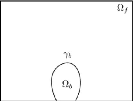
To clearly illustrate the problem, we take a bubble rising from the bottom of the container filled with fluid as an example. The physical setting of the two phase problem is depicted in the Figure 2.1, where Ω_b and Ω_f denotes gas and fluid, respectively.

Figure 2.1: Physical setting

5

(21)

2.2 Fluid Model: Navier-Stokes Equation

Let Ω_t ∈R² be the fluid domain with boundary Γ_t at time t ∈[0, T]. The Navier-Stokes equation for incompressible flow in moving domain can be written as

ρ ∂u

∂t +u· ∇u−f

− ∇ ·σb =0, in [

t∈(0,T)

Ω_t× {t}, (2.1)

∇ ·u=0, in [

t∈(0,T)

Ωt× {t}, (2.2) whereρ,uandfare the density, velocity and the external force, respectively.

We consider only gravityg as an external force. The stress tensorσb can be represented as

σ(p,b u) =−pI+ 2µε(u),

wherepis pressure,Iis the identity tensor,µis viscosity,ε(u) is the strain- rate tensor,

ε(u) = 1

2((∇u) + (∇u)^T).

The initial condition consists of a specified divergence-free velocity field u(x,0) =u₀,

and hydrostatic pressure

p(x,0) =P0+ρgh,

where P0 is atmospheric pressure, g is gravitational acceleration, and h is the depth.

The following boundary conditions are prescribed in general, u=gon (Γt)g,

n·σ=hon (Γt)h, (2.3)

where (Γ_t)_g and (Γ_t)_h are complementary subsets of the boundary Γ_t, n is the unit normal vector, g and h are given functions. Specific boundary conditions arise based on the fact that the boundary of the fluid domain Ω_f is moving, i.e., interface γ_b. We consider interface γ_b as a thin membrane that has mass and its motion is described by the Newton’s second law,

ma=F mdv

dt =σb·n+σκn−f_{f r},

(22)

where the third term of the right-hand side,ff r is the friction force. The first and second terms are the influence from the fluid and interface, respectively.

Writing out the components of stress tensor σb and the proportionality of the friction force to the velocity,

mdv

dt =−pI·n+ 2µ(u)·n+σκn−Cv

where C is a constant. In this case, we assume that Cm and that both the membrane and the fluid are composed of the same material, we obtain

Cv=−pI·n+σκn, (2.4)

which implies that by the absence of the pressure term, the motion of the interface γb according to mean curvature flow.

At this stage, we have the boundary condition on the interface. We need another boundary condition on the moving triple line as free boundary in this problem. Based on what we got in (2.4), the interface evolves according to mean curvature flow. Such kind of motion is derived as the gradient flow of surface energy. Thus, we consider a system that describes the evolution of triple junction under gradient flow of surface energy as explained in the next section.

2.3 Interface Model: Equations of Triple Junction

We write the total surface energy of a curve network and compute its first variation to get the normal velocity for each interface and the condition that has to be satisfied at triple junction. In particular, we consider three evolving curvesγ_i(s) = (γ_i1(s), γ_i2(s)),s∈[p_i, q_i], i= 1,2,3, which lie inside a fixed smooth region Ω ofR², meet the outer boundary∂Ω at a right angle and get together at a triple junctionx_{T L}=γ_i(q_i). Each curve has different surface tension σ_i.

Then the surface energy of all curves is given by

L(γ) =

3

X

i=1

Z

γi

σidl=

3

X

i=1

Z qi

pi

σi |γ_i⁰(s)|ds=

3

X

i=1

Z qi

pi

σi

q

(γ_i1⁰ )²+ (γ_i2⁰ )²ds

(23)

Figure 2.2: Triple Junction

The gradient flow of surface energy can be found from its variation. For a smooth vector fieldϕ= (ϕ₁, ϕ₂) vanishing near the boundary ∂Ω,

d

dL(γ+ϕ(γ))

= d d

3

X

i=1

Z qi

pi

σ_i |γ_i⁰+ d

ds(ϕ(γ))|ds

= d d

3

X

i=1

Z qi

pi

σi

s

γ_i1⁰ +d

ds(ϕ1(γ)) 2

+

γ_i2⁰ +d

ds(ϕ2(γ)) 2

ds

= d d

3

X

i=1

Z _q_i

pi

σ_i q

(γ⁰_i1+(ϕ₁(γ))⁰)²+ (γ_i2⁰ +(ϕ₂(γ))⁰)²ds

=

3

X

i=1

Z _q_i

pi

σ_iA⁻¹²

γ_i1⁰ (ϕ₁(γ))⁰+ (ϕ₁(γ))⁰2

+γ_i2⁰ (ϕ₂(γ))⁰+ (ϕ₂(γ))⁰2

(24)

where A= (γ⁰_i1+(ϕ1(γ))⁰)²+ (γ_i2⁰ +(ϕ2(γ))⁰)² d

dL(γ+ϕ(γ))|₌₀=

3

X

i=1

Z _q_i

pi

σ_i(γ_i1⁰ (ϕ1(γ))⁰+γ_i2⁰ (ϕ2(γ))⁰) p(γ_i1⁰ )²+ (γ⁰_i2)² ds

=

3

X

i=1

Z _q_i

pi

σ_iγ_i⁰·(ϕ(γ))⁰

|γ_i⁰| ds

=

3

X

i=1

Z qi

pi

σ_it_i·(ϕ(γ))⁰ ds

=

3

X

i=1

σ_it_i·ϕ(γ(s))|^q_s=pⁱ

i− Z qi

pi

σ_iϕ(γ)·t⁰_i ds

=

3

X

i=1

σ_it_i·ϕ(x_{T L})− Z

γi

σ_iϕ(γ)·t⁰_i 1

|γ_i| dl

=

3

X

i=1

σ_it_i·ϕ(x_{T L})− Z

γi

σ_iκ_in_i·ϕ(γ) dl

where the tangential vector ti, curvatureκi and outer normalni of curveγi

are given by t_i= γ_i⁰

|γ_i⁰|, κ_i=−γ⁰_i1γ_i2⁰⁰ −γ_i2⁰ γ_i1⁰⁰

|γ_i⁰|³ , n_i = 1

|γ_i⁰|(γ_i2⁰ ,−γ_i1⁰ ).

From this result, the motion by gradient flow satisfies 1. the normal velocity of interface

vi=σiκi. (2.5)

2. condition at triple junction

3

X

i=1

σ_it_i= 0. (2.6)

The junction condition (2.6) is the balance of forces which is well-known to be equivalent to the Young’s law

sinθ1

σ1

= sinθ2

σ2

= sinθ3

σ3

,

(25)

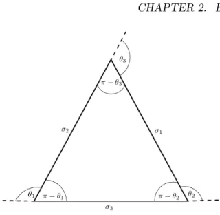
Figure 2.3: Relating surface tensions to junction angles.

whereθ₁, θ₂, θ₃ are the angles at the junction as be described in Figure 2.2.

Note the connection of the above formula to the triangle in Figure 2.3. Using the law of cosines, we obtain the junction angles as in [26]:

cos(π−θ1) = σ₃²+σ₂²−σ₁² 2σ2σ3

, cos(π−θ₂) = σ₁²+σ₃²−σ₂²

2σ₁σ₃ , (2.7)

andθ₁+θ₂+θ₃= 2π.

Note that we can compute the stable angles for any given triple of surface tensions, as long as the triple satisfies the triangle inequality.

2.4 Coupling Strategy

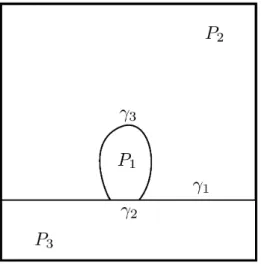
In this section, we summarize the coupling strategies in our case. We treat the problem as depicted in the Figure 2.1 by considering three-phase case as in Figure 2.4. We add solid as an additional phase which does not change the original setting since the solid interface is straight and thus it will not move.

We do so from the beginning in order to be able to suitably treat triple line motion based on the interface model in Section 2.3. Here, Pi, i = 1,2,3 denotes the i-th phase. In particular, P1, P2, P3 represents gas, fluid and solid, respectively.

(26)

Figure 2.4: Physical setting

The interface and fluid models are coupled at interfaceγ3 through pressure pacting from the fluid on the interfaces and by the fact that the interfaces determine the domain for fluid motion. Based on the conditions that we got from the previous sections, the coupling problem can be formulated as follows,

v₃ =σ₃ κ₃+p, at γ₃(t),

3

X

i=1

σiti = 0, at (xT L)(t), ρ

∂u

∂t +u· ∇u−f

− ∇ ·(−pI+ 2µε(u)) =0, in [

t∈(0,T)

P2(t)× {t},

∇ ·u=0, in [

t∈(0,T)

P₂(t)× {t}.

Here, xT L are the triple points and P2(t) ⊂ R² is the fluid domain with boundary given by Γt = γ1(t)∪γ3(t)∪∂Ωt, where ∂Ωt is the part of the external boundary which has contact with the fluid.

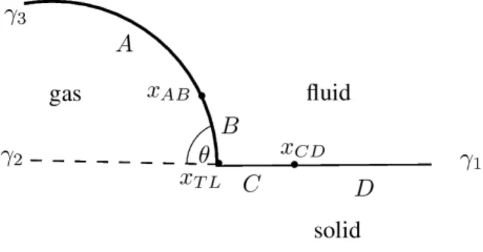
In this problem, we have to apply appropriate boundary conditions which can handle moving triple line. At gas-fluid interface, we apply free-slip boundary condition, while at solid-fluid interface we apply no-slip boundary condition. The discrepancy of these conditions at triple line causes a nonphysical divergence of the hydrodynamic pressure and of the viscous dis- sipation at triple line [43, 44]. To avoid this discrepancy, we use some kind

(27)

of slip-boundary condition. We smoothly connect these two conditions at triple line by using smoothing length as in the formula below.

Figure 2.5: Vicinity of triple line

• If x=x_{T L}

u·t_b = 0, u·n_b=v,

u·t=vsinθ, u·n=vcosθ,

• If x∈A

tb·σ·nb= 0, u·nb =v,

• If x∈B

γ tb·σ·nb =β(u·tb),u·nb =v,

• If x∈C

u·t=α vsinθ,u·n=α vcosθ,

• If x∈D

u·t= 0,u·n= 0,

where β = |x_AB −x|, γ = |x_{T L} −x|, α = _|x^|x−x^CD^|

T L−x_CD| are the smoothing lengths,uis the velocity of the fluid,vis the normal velocity of the interface, t_b, t, n_b, nare tangential and normal vectors ofγ₃ and γ₁, respectively.

Note that in the coupling problem, volume preservation is essential for stable computation. In the numerical method, we incorporate the volume constraint in the interface model.

(28)

Numerical Method

3.1 Numerical Solution of Interface Model:

BMO Algorithm with Arbitrary Surface Tensions

The problem of simulating the motion of interfaces with triple junction according to some curvature-dependent speed arises in many applications, e.g., grain growth [9], image processing [10], multiphase flow [11]. Equal surface tensions lead to symmetric triple junction, which is well-known as the symmetric Herring condition (interfaces meeting at 120^◦). On the other hand, arbitrary surface tensions lead to nonsymmetric triple junctions.

To treat such motions, several methods have been developed. As has been mentioned in the introduction, Bronsard et al. [23] uses the reaction- diffusion equation

u_t=ε∆u−1

ε∇_uW(u), (3.1)

to model triple junctions. Here, ε > 0 is a small parameter and W is a well potential, a non-negative function which has three minima for the three-phase case. This so-called phase-field method represents the phase boundary as an interfacial layer. In [23], the authors showed that the interfaces in the solution of (3.1) move with a velocity proportional to the curvature of the interface and in its sharp interface limit (ε→ 0), one obtains the Young’s law at the junction. However, this method has difficulties in the numerical solution when ε <∆x, where ∆x is the spacing grid. The only remedy to these difficulties is to take ^∆x_ε 1, which is impractical numerically [17]. Moreover, it is also necessary to appropriately determine parameters of the well-potential function which amounts to a complicated

13

(29)

minimization problem. Garcke et al. [24] performed numerical simulations for a multiphase field model and showed that for suitably chosen parameters (determined based on numerical experiments), numerical results agree with the formal asymptotic expansion of [25] and yield the correct motion.

On the other hand, Zhao et al. [41] developed a numerical algorithm capturing the interfaces based on the level set method of Osher et al. [42].

This method is able to deal with topological singularities and nonsmooth data. Moreover, it can be extended to the multiphase setting by introducing as many level set functions as there are phases and imposing additional constraint on the constrained flow problem so that the level sets do not overlap or create vacuums. However, such a constraint has an unwanted influence on the motion and the volume of phases is not sufficiently controlled by the method.

Merriman, Bence and Osher [17] introduced the BMO method, an implicit scheme for realizing interfacial motion by mean curvature for symmetric junctions, which alternately diffuses and sharpens characteristic function for each phase region. For two-phase case, it has been shown that the method converges to motion by mean curvature [18, 19, 20]. Ruuth [12]

generalized the BMO method to nonsymmetric triple junctions by replacing the thresholding step with a new decision, i.e., by using a projection triangle.

This generalized method also allows for normal velocity equal to a positive multiple of the curvature of the interface plus the difference in bulk energies for prescribed junction angles. Svadlenka et al. [11] reformulated the BMO algorithm in vector-valued formulation for multiphase motion. This vector- valued formulation is essential for implementing constraints and for dealing with more general motions. However, it is restricted to the symmetric case.

Mohammad et al. [21, 22] improved the symmetric multiphase BMO algorithm of [11] by introducing a signed distance vector-valued function.

In this work, we consider three evolving curves meeting at a junction and having arbitrary surface tensions. We achieve the simulation of such a triple junction by generalizing the two main ingredients of the method in [11]:

the reference vectors (corresponding to the positions of wells in the phase- field method) and the diffusion step. Moreover, we improve the scheme by including a modification of the projection step in [12]. The developed method is applicable to constrained motions.

3.1.1 Vector-valued BMO

The basis of our method is the vector-valued BMO algorithm [11]:

1. Define reference vectorsp_i of dimension two, each corresponding to a

(30)

phase Pi fori= 1,2,3.

2. Given a partitionPi,i= 1,2,3, set u0(x) =p_i forx∈Pi. 3. Repeat

• Solve the vector-valued heat equation with initial conditionu₀: u_t(t, x) = ∆u(t, x) for (t, x)∈(0,∆t]×Ω,

∂u

∂n(t, x) = 0 on (0,∆t]×∂Ω.

• Updateu0 by identifying the reference vector which is closest to the solutionu(∆t, x):

u₀(x) =p_j,

where p_j·u(∆t, x) = maxi=1,2,3p_i·u(∆t, x).

This redistribution of reference vectors determines the configuration of each phase after time ∆t.

Note that this algorithm deals only with symmetric junctions, the use of symmetric reference vectors and simple heat equation in the diffusion step.

However, for arbitrary junction angles, this setting is not sufficient and has to be generalized. We will do so in the following two sections.

3.1.2 Junction Stability

Consider three straight lines meeting at the origin with the given stable angles as in Figure 3.1. The fact that this configuration is stable will yield a condition on the selection of reference vectors for the BMO algorithm.

The triple junction does not move ifu(t,0,0) =0 for all t >0, where u is the solution of the heat equation. This means

1 4πt

3

X

i=1

p_i Z

R²∩Pi

exp(−|x|²

4t ) dx=0.

Since by radial symmetry, we can compute the integral of the wedge P_i as Z

Pi

e^−|x|²dx= θi

2,

(31)

Figure 3.1: Configuration of a stable junction.

we get

θ₁p₁+θ₂p₂+θ₃p₃ =0. (3.2) The above relation is a one-dimension higher BMO analogue of Young’s law (2.6) in the sense that the reference vectors p_i are distributed in the whole phase regions P_i and, thus, the equilibrium condition is related to area integrals, which results in weights equal to junction angles.

The vector equation (3.2) and the condition obtained in the next section that the lengths ofp_i, i= 1,2,3, must be equal, form a systems of equations for the components ofp_i:

θ1p¹₁+θ2p¹₂+θ3p¹₃= 0 θ₁p²₁+θ₂p²₂+θ₃p²₃= 0 (p¹₁)²+ (p²₁)²= 1 (p¹₂)²+ (p²₂)²= 1 (p¹₃)²+ (p²₃)²= 1

Since the reference vectors are determined up to rotation and scaling, we can choose one reference vector arbitrarily, e.g., we set p₃ = (1,0). This closes the system and its solution can be written as

(32)

p¹₁= 1− 2π θ1θ3

(π−θ2), p²₁=± 2

θ₁θ₃

pπ(π−θ1)(π−θ2)(π−θ3), p¹₂= 1− 2π

θ₂θ₃(π−θ₁), p²₂=∓ 2

θ2θ3

pπ(π−θ₁)(π−θ₂)(π−θ₃).

(3.3) The possible choices for the sign of the second component follow from the invariance of the reference vectors with respect to flipping.

3.1.3 Interface Velocity

Here, we study the modification of the original BMO algorithm yielding the correct interface velocities v_i=σ_iκ_i. The idea is to consider, instead of the heat equation, the general diffusion system











u¹_t +du²_t =a∆u¹+b∆u², du¹_t+eu²_t =b∆u¹+c∆u²,

u¹ u²

!

(t= 0) = u¹₀ u²₀

! ,

(3.4)

and determine its coefficients a, b, c, d, e, so that we obtain the desired interface velocities. We will show that this leads to a system of nonlinear equations fora, b, c, d, e. Moreover, we check that the change of the underly- ing diffusion system does not influence the arguments of the previous section on junction stability.

Note that we restrict our considerations to symmetric coefficient ma- trices. This is due to the fact that in order to incorporate phase-volume preservation, we use the variational structure of the system in an essential way (see subsection 3.1.6).

The system (3.4) can be rewritten in the form

˜

u_t=A∆˜u, where

˜ u=

u˜¹

˜ u²

= 1 d

d e u¹ u²

,

(33)

and

A= 1 e−d²

ae−bd b−ad be−cd c−bd

.

We assume that A is positive definite and diagonalize it in the following form

A=KΛK⁻¹ with Λ =

λ1 0 0 λ₂

. The eigenvalues ofA are given by

λ_1,2 = ae+c−2bd±r 2(e−d²) , wherer=p

(ae−c)²+ 4(ad−b)(cd−be).

Hence, we get the matrixK consisting of eigenvectors as K= 1

2r

ae−c+r 2(ad−b) 2(be−cd) ae−c+r

. The original problem is transformed into











w¹_t =λ₁∆w¹, w²_t =λ2∆w²,

w¹ w²

!

(t= 0) = w₀¹ w₀²

!

=M u¹₀ u²₀

! ,

(3.5)

where w¹

w²

=M u¹

u²

,withM =K⁻¹ 1 d

d e

.

The solution to the transformed problem (3.5) in the whole R² is wⁱ(t, x) = 1

4πλit Z

R²

w₀ⁱ(ξ)e⁻

|x−ξ|2

4λit dξ, i= 1,2, (3.6) where

wⁱ₀|_P_j = ((Mu0)|_P_j)ⁱ = (Mp_j)ⁱ, i= 1,2, j= 1,2,3.

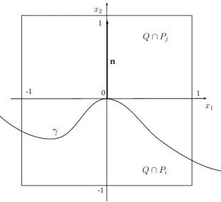
Now, let us calculate the velocity of the interface for the above diffusion system. We consider a point on the interfaceγ =∂P_ij between phaseP_iand Pj. We translate and rotate the coordinate system so that the chosen point lies in the origin and the outer normal at the point agrees with the positive x₂-direction. We define Q = [−1,1]×[−1,1]. Then the normal velocity v

(34)

Figure 3.2: Configuration of the interface.

of the interface is found from the relation, expressing the condition on the interface position along the x₂-axis after time t, i.e.,

u(t,0, vt)·(p_i−p_j) = 0. (3.7) We can write the solution of the transformed problem (3.5) as

w(t,0, vt) =





 1 4πλ1t

R

R²w₀¹(ξ)e⁻

|ξ−(0,vt)|2 4λ1t dξ 1

4πλ₂t R

R²w₀²(ξ)e⁻

|ξ−(0,vt)|2 4λ2t dξ





 .

By the techniques in [18] and [27], we get 1

4πλ1t Z

Q∩Pi

e⁻

|ξ−(0,vt)|2

4λ1t dξ= 1 2+

√ t 2√

πλ1

(λ1κ−v) +O(t³²), (3.8)

where κ is the curvature of ∂P_ij at the origin. Hence, we have for l= 1,2,

(35)

and someC >0, w^l(t,0, vt)

= w₀^l|_P_i 4πλlt

Z

Q∩Pi

e⁻

|ξ−(0,vt)|2

4λlt dξ+ w₀^l|_P_j 4πλlt

Z

Q∩Pj

e⁻

|ξ−(0,vt)|2

4λlt dξ+O(e⁻^C^t)

= w^l₀|_P_i 1

2+

√t 2√

πλl

(λlκ−v)

+w^l₀|_P_j 1

4πλlt Z

R²

e⁻

|ξ−(0,vt)|2 4λlt dξ

−w^l₀|_P_j 1

2+

√ t 2√

πλ_l(λlκ−v)

+O(t³²)

= w^l₀|_P_i 1

2+

√t 2√

πλ_l(λ_lκ−v)

+w^l₀|_P_j 1

2−

√t 2√

πλ_l(λ_lκ−v)

+O(t³²)

= w^l₀|_P_i +w^l₀|_P_j

2 + w₀^l|_P_i−w₀^l|_P_j 2

√t

√πλ_l(λ_lκ−v) +O(t³²).

We obtain from (3.7) the identity M⁻¹

Mp_i+p_j

2 +

√t

√πDMp_i−p_j 2

·(p_i−p_j) =O(t³²), where

D=







√1

λ₁(λ₁κ−v) 0

0 1

√λ₂(λ₂κ−v)





.

Notice that if the first dot product on the left-hand side does not vanish, then the order in time of the equation does not match. This leads to the condition (p_i +p_j)·(p_i −p_j) = 0, meaning that the lengths of reference vectors have to be equal (see subsection 3.1.2). Then we obtain

(p_i−p_j)^TM⁻¹DM(p_i−p_j) =O(t), which is, up to orderO(t), equivalent to

µ1

pλ1κ− 1

√λ₁v

+µ2

pλ2κ− 1

√λ₂v

= 0, where

µ₁= m₁₁m₂₂(p¹_ij)²−m₁₂m₂₁(p²_ij)²+ (m₁₂m₂₂−m₁₁m₂₁)p¹_ijp²_ij, µ2= −m12m21(p¹_ij)²+m11m22(p²_ij)²−(m12m22−m11m21)p¹_ijp²_ij,

(36)

with p_ij =p_i−p_j and m11, m12, m21, m22 denote the entries of the matrix M. Finally, we get the velocity of interface γ_k (k6=i, j) in the form

v_k = µ1

√λ1+µ2

√ λ₂ µ2

√

λ1+µ1

√ λ2

pλ₁λ₂κ_k.

Since there are only three types of interfaces, it is expected that we need only three parameters in order to design the velocities. Hence, it is reasonable to try to set d= 0, e= 1, so that our diffusion system becomes

u_t=A∆u, (3.9)

withA= a b

b c

.We could have done so from the beginning of this section but, as we will see below, the resulting nonlinear system fora, b, cis hard to analyze theoretically, which led us to keep the parametersdand eas a last resort in case the three-parameter system cannot be solved. In this case, we get the interface velocities

v_k= µ₁(a+c+r) + 2µ₂√ ac−b² µ2(a+c+r) + 2µ1

√ ac−b²

pac−b²κ_k, (3.10) where

r=p

(a−c)²+ 4b²

µ1 = [(a−c+r)(p¹_i −p¹_j) + 2b(p²_i −p²_j)]², µ₂ = [2b(p¹_i −p¹_j)−(a−c+r)(p²_i −p²_j)]².

From (3.10) and (2.5), we have a nonlinear system consisting of three equations for the coefficients a, b and c, which is solved numerically. First, we simplify it by setting

x = α+p β²+ 1 pα²−β²−1, y = β+p

β²+ 1, z = bp

α²−β²−1,

where α = (a+c)/(2b) and β = (a−c)/(2b). Then the above system in terms of x, y, z becomes

(p¹_ijy+p²_ij)²x+ (p¹_ij −p²_ijy)² (p¹_ij−p²_ijy)²x+ (p¹_ijy+p²_ij)²z=σk

(37)

for (i, j, k) = (2,3,1),(1,3,2),(1,2,3). We take any two equations from this system and solve forx, zanalytically, which is possible, since the corresponding equation is quadratic. Due to this fact, we get two different solutions for x, z. For each such pair of x, z, we use a numerical method (such as Newton’s method) to find the rooty of the remaining equation. There may exist several roots fory. For each such combination ofx, y, zwe recoverα, β andb by

α= (x²+ 1)(y²+ 1)

2(x²−1)y , β = y²−1

2y , b=±x(y²+ 1) (x²−1)y.

The coefficients a and c are then obtained easily. The number of cases double because of two possible signs forb. All triples (a, b, c) obtained in the described way are then checked if they solve the system and the appropriate triple is selected.

Since the nonlinear system is very complicated, we were not able to prove the unique existence of solution using analytical methods, such as fixed point theory. However, in using the above method, we can always find a solution, except whenb= 0 which occurs when two of the surface tensions are equal.

In that case, the system simplifies in such a way that it can be solved fully analytically.

Table 3.1: Coefficients of Diffusion System in some Cases (σ1, σ2, σ3) (a, b, c)

(1,1,1) (1,0,1)

(1,1.5,1) (1.43773,0.19887,0.86481) (1.,1.8,1.) (1.76785,0.18910,0.68793) (1.5,0.75,1.) (1.43308 -0.25468 0.67283)

(1.5,1.,1.) (1.43773,-0.19887,0.86481) (1.5,1.25,1.) (1.50944,-0.10082,0.96859) (1.5,2.,1.) (2.02618,0.12516,0.89890 ) (1.8,1.,1.) (1.76785,-0.18909,0.68793 ) (2.,1.5,1.) (2.02618,-0.12516,0.89890 )

(2.,2.,1.) (2.2408,0,1 )

Remark. For the initial condition in Figure 3.1, at the triple junction we

(38)

have

wⁱ(t,0) = 1 4πλit

Z

P1

+ Z

P2

+ Z

P3

w₀ⁱ(ξ)e⁻

|ξ|2 4λitdξ

= 1 π

θ1

2wⁱ₀|_P₁ +θ2

2 w₀ⁱ|_P₂ +θ3

2w₀ⁱ|_P₃

. Therefore,

w(t,0) = 1

2πM(θ₁p₁+θ₂p₂+θ₃p₃).

For junction stability, we require u(t,0) =M⁻¹w(t,0) =0. This condition is equivalent to

θ₁p₁+θ₂p₂+θ₃p₃=0, which is in agreement with (3.2).

This result shows that no matter how we change the diffusion equation, the stability condition (3.2) will not be affected. Hence, the selection of reference vectors can be done independently of the diffusion equation.

3.1.4 Correction by Projection Triangle

In the previous sections, we have derived an extension of the vector-valued BMO algorithm to include the case of nonsymmetric junctions and general interface velocities. We have shown that, for a suitably selected diffusion system, if an interface point is sufficiently far from the junction, the interface velocity at that point will satisfy the desired formula vi = σiκi, and that, for a suitably selected reference vectors, the junction will be stationary for the initial configuration of three straight lines meeting at the junction with stable contact angles.

However, the above analysis does not address the close vicinity of the triple junction. In fact, by formal calculations it can be made clear (see Appendix 3.1.8) that the correct interface velocity is obtained only with an exponentially decreasing error with respect to the distance of the considered interface point to the junction. Indeed, numerical tests proved that the stable configuration consisting of three straight lines slightly curves in the neighborhood of the junction. This fact produces errors in the angles of the moving junction.

Therefore, we include a correction step based on the notion of a projection triangle given by Ruuth [12]. The idea is to first investigate how the stable configuration of three straight lines deforms, and use this information

(39)

to project the phase regions back into the correct position in each step of the BMO algorithm. For details of the construction of the projection triangle we refer to [12].

The original method in [12] uses the scalar setting, i.e., it diffuses sep- arately characteristic functions for each of the three phase regions of the stable configuration (Figure 3.1) which yields three values of diffused function at every point in the domain. These three values are positive and sum up to one, thus, taken as points in R³, which lie inside a triangle on a hyperplane of R³. The straight lines of the stable configuration are mapped on the triangle as dividing curves. In order to relate our vector- valued formulation to the construction in [12], we introduce the functions for (i, j, k)∈ {(1,2,3),(2,3,1),(3,2,1)},

f_i(t, x) = u(t, x)·(p_j +p_k)−1−p_j·p_k

(p_i−p_j)·(p_j+p_k) , (3.11) Note that (3.11) is a generalization of the function w_i(t, x) in [11], Section 2.2.2, for general reference vectors (3.3). Since u(0, x) =p_i forx∈Pi, one can easily check that

f_i(0, x) =χ_i(x), i= 1,2,3, whereχ_i is the characteristic function of phase regionP_i.

However, the advantage of our vector-valued approach is that we do not have to perform separate diffusions and subsequently identity the hyperplane x₁+x₂+x₃ = 1. It is sufficient to diffuse the vector-valued initial condition as in Figure 3.1 and record the images of the straight lines. In this way, we obtain a projection triangle that can be used directly for the function u in the BMO algorithm.

We summarize the construction of the projection triangle in the generalized vector-valued formulation. Given an angle configurationθ1, θ2, θ3, we perform the following steps:

1. Define the lines (in polar coordinates)

`12={(r,1

2θ1) :r >0},

`₁₃={(r,−1

2θ₁) :r >0},

`₂₃={(r,1

2θ₁+θ₂) :r >0}, and regions P₁, P₂, P₃, as in Figure 3.1.

(40)

2. Setu0(x) =p_i forx∈Pi.

3. Apply the diffusion (3.4) to the initial condition u0 for a timeτ ≤∆t, where ∆t is the BMO time step.

4. Map the values of the solution of step 3 along each line `ij onto the projection triangle to form the dividing lines ˜`_ij:

`˜ij ={u(τ, x) :x∈`ij}.

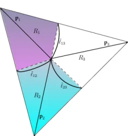
Figure 3.3: Projection triangleT in vector-valued setting.

Notice that the values of the diffused functionufall inside the triangleT formed by the vectors p₁,p₂,p₃ (Figure ). Moreover, because of (3.2), the dividing lines ˜`12,`˜13,`˜23 will always meet at the origin which corresponds to the circumcenter of T, and they approach the midpoints of edges of T on their other ends. This is in contrast to the projection triangles in [12], where the position of the junction shifts and the shape of dividing lines is distorted, especially for junction angles strongly deviating from the Herring symmetric case. This fact helps significantly to make the numerical computations stable, especially for the volume-preserving problem.

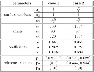
Figure 3.4 shows the resulting projection triangles for the 150^◦−90^◦− 120^◦ junction and the 135^◦−90^◦−135^◦ junction. Since these two cases will be used in numerical tests, we list the coresponding parameters in Table 3.2.

As it sometimes happens in the numerical computations that the values of

(41)

Table 3.2: Numerical parameters for case 1 and case 2

parameters case 1 case 2

surface tensions

σ₁ ¹₂

√ 2 2

σ₂ 1 1

σ3

√ 3 2

√ 2 2

angles

θ₁ 150^◦ 135^◦

θ₂ 90^◦ 90^◦

θ3 120^◦ 135^◦ coefficients

a 0.881 0.954

b 0.262 0.127

c 0.656 0.639

reference vectors

p₁ (-0.8,-0.6) (-0.777,-0.628) p₂ (0,1) (-0.333,-0.943)

p₃ (1,0) (1,0)

the function u fall out of the projection triangle, we extend the dividing curves by straight lines connecting the junction to the midpoints of the edges.

(a) (b)

Figure 3.4: Projection triangle for (a) 150^◦−90^◦−120^◦and (b) 135^◦−90^◦− 135^◦ triple junctions.

Remark. There is a close relation between the BMO algorithm and a splitting method for the phase-field equation (3.1), which repeats the following steps:

1. Diffuse for a time ∆t

ut=ε∆u, with initial condition u(0, x) =u₀.

(42)

2. Solve

u_t=−1

εW⁰(u), (3.12)

with initial condition u(∆t, x).

One can see that (3.12) corresponds to the thresholding step in BMO in the sense that the solution asymptotically separates into three regions with values equal to the minima of W. The dividing lines between these regions are the separatrices for the well potential W. The well potential can be chosen as in [24] but, as mentioned earlier, it is not easy to calibrate its parameters since they are not given by an explicit formula.

3.1.5 Generalized Vector-valued BMO Algorithm

In this subsection, we summarize the above deliberations into a generalized vector-valued BMO scheme. First we present the basic version of the BMO algorithm and then comment on the method of incorporating the volume constraint. The generalized vector-valued BMO for three-phases motion is as follows:

1. For given surface tensions, calculate junction anglesθi by (2.7).

2. Define reference vectors p_i according to formula (3.3).

3. Find the solution a, b, c of (3.10) and setA= a b

b c

.

4. Construct projection triangle according to the algorithm in subsub- section 3.1.4.

5. For a given three phase initial configuration P1, P2, P3, set u₀(x) =p_i, x∈P_i.

6. Repeat until desired time

• Solve the diffusion system

u_t=A∆u for (t, x)∈(0,∆t]×Ω, (3.13)

∂u

∂n = 0 on (0,∆t]×Ω, u(0, x) =u₀(x) in Ω.

(43)

• Threshold according to the projection triangle defined in step 4, i.e.,

u₀(x) =p_i if u(x)∈R_i, i= 1,2,3, where Ri are the regions in Figure .

The modified diffusion system is solved by using vector-type discrete Morse flow (DMF) [28], i.e., at each step we solve (3.13) by discretizing time ∆t=h×N and successively minimizing the following functionals for n= 1, .., N overH¹(Ω;R²):

Jn(u) = Z

Ω

a

2|∇u¹|²+b∇u¹· ∇u²+ c

2|∇u²|² dx +

Z

Ω

|u−un−1|² 2h

dx. (3.14)

We approximate the functional (3.14) by using piecewise linear finite elements. The minimizers are found by steepest descent method.

3.1.6 Generalized Vector-valued BMO Algorithm with Vol- ume Constraint

The minimization formulation of the vector-valued algorithm allows the in- clusion of volume constraints via penalization. In particular, instead of the functionalJn in step 6, we minimize

Fn(u) =Jn(u) +1

3

X

i=1

|V_i−meas(P_i^u)|².

Here > 0 is a small penalty parameter, V_i is the prescribed volume of regionPi and the volumes corresponding tou are obtained from the sets

P_i^u={x∈Ω;u(x)∈R_i}.

This means that we have to employ the projection triangle each time we evaluate the functionalF_n.