Comparison of numerical methods for 1-D hyperbolic-type problems with free boundary

(1)

Comparison of numerical methods for 1‑D

hyperbolic‑type problems with free boundary

著者ファイザルマホロス

著者別表示 Faizal Makhrus journal or

publication title

博士論文本文Full 学位授与番号 13301甲第4315号

学位名博士（理学）

学位授与年月日 2015‑09‑28

URL http://hdl.handle.net/2297/43828

(2)

Dissertation

Comparison of numerical methods for 1-D hyperbolic-type problems with free boundary

１次元双曲型自由境界問題の数値解法の開発と評価

Graduate School of

Natural Science and Technology Kanazawa University

Division of Mathematical and Physical Sciences Course in Computational Science

School registration No.: 1223102012

(3)

Abstract

In this research, we study a 1-D hyperbolic-type problem with free boundary. We consider a physical model that is the motion of a piece of tape being peeled off from a surface. The graph of the solution shows the shape of the tape, which displays contact angle dynamics at the free boundary (the lo- cation of peeling). Therefore, the second derivative of the solution becomes a delta function which imparts a slight difficulty. Under some assumptions, this problem can be solved numerically by the fixed domain method. Al- though, this method has high accuracy, it cannot be applied in some cases such as a problem where the free boundary point appears or disappears.

Hence, other numerical methods are chosen for solving regularized problem, i.e., the delta function is approximated by a smoothing function. The numerical methods are: two types of finite difference methods, the finite element method, and discrete Morse flow. In this paper, the error of the regularized problem compared to the original problem is calculated. Since the choice of the parameter for smoothing function is important for the accuracy, we pro- pose a formula to approximate the optimal parameter in order to minimize the error. This formula is verified by some experiments and we find that it can approximate the optimal parameter. In addition, based on comparisons between the numerical methods, we find that finite difference methods have better performance than the other methods.

(4)

List of Figures

5.1 Exact solution (5.7) . . . 25

5.2 Estimation from above of the total error for explicit method 2 28 5.3 The errors of explicit method 2 for cases 1-6 . . . 29

5.4 The errors of free boundary point of cases 1-6 . . . 30

5.5 The errors of solution for case 1-4 with different gradient with ∆x= 0.000625 . . . 31

5.6 the lower and upper bound of optimal ε for cases 1-4 . . . 32

5.7 The range of constant C for cases 1-4 with different ∆x . . . . 33

5.8 Comparison of smoothed characteristic functions . . . 34

5.9 Error of numerical methods and exact solution of equation (5.7) 36 5.10 Eu atτ = 9 of cases 1-4 . . . 38

5.11 The numerical solutions of case 7 . . . 40

5.15 Error in case 7 at u(2.5,5) . . . 42

(7)

Chapter 1 Introduction

In this study, we treat a physical model which can be considered as peeling tape attached to a surface. Imagine that there is a piece of tape pasted to a surface and it is peeled off from its edge smoothly. This model can be described as a stationary point of the following action integral in a suitable function space:

J(u) = Z τ

0

Z

Ω

(1

2|∇u|²− 1

2(u_t)²χ_u>0+Q²

2 χ_u>0)dxdt, (1.1)

whereuis a scalar function (0, τ)×Ω7→Rwhich represents the shape of the tape, Q is a given positive constant, Ω is a domain in R^d(d ≥1), and χ_u>0 is a characteristic function of the set {(x, t) : u(x, t) > 0}. The following Euler-Lagrange equation can be derived from functional (1.1) under certain assumptions [2]:

(u_tt= ∆u in (Ω×(0, τ))∩ {u >0},

|∇u|² −(u_t)² =Q² on (Ω×(0, τ))∩∂{u >0}. (1.2) When d= 1, under certain conditions, [4] showed that the existence and the uniqueness of its solutions are obtained locally.

On the other hand, the following equation is equivalent to (1.2) (see Subsection 2.1):

χ{u>0}u_tt = ∆u− Q²

|Du|H^db∂{u >0} in Ω×(0, τ), (1.3)

(8)

whereH^disd-dimensional Hausdroff measure andDu= ∂u

∂x₁, . . . ∂u

∂x_d,∂u

∂t

! . On the other hand, we consider the following equation as the approximation of problem (1.3)

χ_{u>0}u_tt = ∆u− Q²

2 (χ^ε)⁰(u) in Ω×(0, τ), (1.4) where χ^ε(u) is an appropriate smoothing function. Equation (1.4) can be used to model not only the simple case of peeling tape but also more advanced free boundary problems such as water droplet attached to a plane, bubble touched the water surface, and other phenomena [3] [5] [7] [8] with constraints applied.

The motivation behind this research is to solve the original problem (1.3) yet it is difficult. Fortunately, [2] introduced the fixed domain method which solved problem (1.2) in 1D which is equivalent to the original problem (1.3) if the solution is non-negative. Fixed domain method has high accuracy.

However, it is difficult to handle such model where the free boundary point appears or disappears. Therefore, we investigate another numerical methods.

We choose a few numerical methods namely:

1. explicit method 1 (spatial central difference and time forward difference)

2. explicit method 2 (spatial and time central difference) 3. finite element method (FEM)

4. discrete Morse flow (DMF).

We choose explicit method 1 and 2 as they are standard methods. Here, explicit method 2 is a standard finite difference method which can be used to analyze the error of the solution of the regularized problem. We choose FEM as it is widely used to approximate solution of hyperbolic-type problem. DMF is chosen since it is used in many hyperbolic-type problem with constraints. These methods are used to solve the regularized problem (1.4), i.e., the measure is approximated by using smoothed characteristic function.

(9)

The second purpose is to investigate how to obtain small error by the selection of the parameter of smoothed characteristic function (ε). Here, we proposed a formula to approximate the appropriate choice of ε (see Section 5.3). The third purpose is to investigate the different kinds of smoothed characteristic function. We consider two types of smoothed characteristic function and compare their influences to the accuracy of the solution in order to get the suitable one (see Section 5.4). The fourth purpose is to compare the numerical methods in order to get the suitable method (see Section 5.5).

The last purpose is to implement more general case such as a model in which the free boundary points attached to a surface are more than one and they appear or vanish during simulation time (see Section 5.6).

In this dissertation, we organize our chapters as: chapter 2 explains the physical model of peeling tape, chapter 3 gives the details of fixed domain method, chapter 4 presents the numerical methods in details, chapter 5 dis- cusses the results of our experiments, and chapter 6 gives the conclusion.

(10)

Chapter 2 Physical model of peeling tape problem

This section explains the physical model of peeling tape on a plane. Suppose there is a thin film adhered to a plane and consider this film as our tape. It is peeled off from the plane and starts to expand along the sticked tape. The region where the tape is peeled or adhered is considered as a domain Ω. We assume that the tape has the same tension γ at any places. The shape of the tape is represented by a function u : Ω→R. The value of u is obtained by the stationary point of this model’s energy.

There are two potential energies in this model

E = Z

{u>0}

γ(p

1 +|∇u|²−1)dx+ Z

{u>0}

(γ− q

γ²+ ˜Q²)dx.

Using Taylor expansion we can get E˜ =

Z

{u>0}

γ

2|∇u|²dx+ Z

{u>0}

Q² 2 dx,

where Q² = ˜Q²/γ. Another energy of this model is kinetic energy

(11)

of the tape is

L(u, t) = Z

Ω

γ

2|∇u|²− ρ

2u²_tχ_u>0+Q² 2χ_u>0

!

dx. (2.1)

The equation of tape evolution within time interval [0, τ] is J(u) =

Z τ 0

Z

Ω

γ

2|∇u|²− ρ

2u²_tχ_u>0+ Q² 2 χ_u>0

!

dxdt. (2.2)

We choose γ =ρ= 1.

From this energy function, the problem can be derived into Euler-Lagrange equation. Assume that the stationary point of equation (2.2) is sufficiently smooth. Let u be the stationary point of (2.2) and u ∈ C⁰(Ω×(0, τ)∩ W^1,2(Ω, τ)), then u satisfies

∆u−u_tt = 0 in {u >0}. (2.3) Moreover, if u∈C²(Ω×(0, τ)∩ {u >0}) and∂{u >0} is inC⁻¹, thenu on the boundary satisfies

|∇u|²−u²_t =Q² on ∂{u >0}. (2.4) The proofs of (2.3) and (2.4) can be seen in [2].

The proof of (2.3) is the first variation of (2.2) with test function ϕ ∈ C₀^∞(Ω×(0, τ)∩ {u >0})

Z t 0

Z

Ω

(∇u∇ϕ−utϕt)dxdt= 0,

that is (2.3). By inner variation, we can obtain (2.4). Now, we consider u ∈ C²(Ω × (0, τ)∩ {u > 0} and it is assumed that the free boundary

∂{u > 0} belongs to C¹. For any η ∈ C₀^∞(Ω×(0, τ);Rⁿ× R) and 0 <

< dist(spt η, ∂(Ω×(0, τ))) such that for small it follows the mapping ψ : Ω ×(0, τ) → Ω×(0, τ) and we define ψ(z) = z +η(z). Here z is a variable of Ω ×R, ie. z_j = x_j(j = 1, . . . , n) and z_n+1 = t. Now, let u(z) =u◦ψ⁻¹(z). Sinceu is stationary point of J it is

d

dJ(u)|₌₀ = 0.

(12)

On the other hand, we calculate J as

J(u) = − Z

Ω×(0,τ)∩{u>0}

h∇hu(Dψ)⁻¹,∇hu(Dψ)⁻¹i|det Dψ|dz.

Here, ∇zf = (fz1, . . . , fzn, fzn−1) and ∇hf = (fz1, . . . , fzn,−fzn−1). h., .i is inner product of Rⁿ⁺¹ and Dψ is Jaccobian matrix of ψ. Therefore,

J(u)−J(u) = Z

Ω×(0,τ)∩{u>0}

h∇_hu,∇_zui+Q² ∇_z.ηdz

− Z

Ω×(0, τ)∩ {u >0}2∇_huDη∇_zudz+o().

By the following equation

∇_z.(ηh∇_hu,∇_zui −2hη,∇_zui∇_hu)

=∇_z.ηh∇_hu,∇_zui −2∇_huDη∇_zu−2ηhη,∇_zui(∆u−u_tt), we get

d

dJ(u)|₌₀ = Z

Ω×(0,τ)∩{u>0}

∇_z. ηh∇_hu,∇_zui −2hη,∇_zui∇_hu+Q²η dz

= Z

Ω×(0,τ)∩∂{u>0}

{(h∇_hu,∇_zuiη−2hη,∇_zui∇_hu).ν +Q²hη, νi}dHⁿ.

Here, Hⁿ isn-dimensional Hausdroff measure. In addition, ν is outward unit normal vector with respect to Ω×(0×τ)∩ {u >0}. Since, ∇_zu=−ν|∇_zu|

then, d

dJ(u)|₌₀ =− Z

Ω×(0,τ)∩∂{u>0}

(h∇_hu,∇_zui −Q²)hη, νidHⁿ.

(13)

define a smooth function called β_ε(s). β_ε(s) ∈ C²(R), β_ε(s) ≥ 0, and satisfies

β_ε(s)











= 0 s≤0,

≤2/ε 0< s < εand |β_ε⁰(s)| ≤ C ε²,

= 0 ε≤s.

It is also that Rε

0 β_εds = 1 and we define B_ε B_ε(u) =

Z u 0

β_ε(s)ds−→

ε→0

(1 in{u >0},

0 in Ω×(0, τ)\{u >0}, which is the smoothing characteristic function of χ_u>0.

We represent energy equation (2.2) J_ε(u) =

Z τ 0

Z

Ω

1

2|∇u|²−χ_u>01

2u²_t +Q² 2 B_ε(u)

!

dxdt. (2.5) By taking the first variation of (2.5), our problem becomes











∆u−χu>0utt=−Q²

2 βε(u) in Ω×(0, τ), u(x,0) = u₀(≥0)

u_t=v₀

u(x, t)|_∂Ω =f(x, t) with f(x,0) =u₀ on∂Ω.

(2.6)

We call this as the regularized problem.

2.1 Derivation of the original problem

In this subsection we show the derivation of (1.3) based on [6]. Let Q_T :=

Ω×(0, τ). We assume u ∈ H²({u > 0})∩C(QT) is solution of (1.2) and satisfies u≥0 and {u >0} ⊂C^0,1. By definition,

(u_tt−∆u)(ϕ) =− Z

QT

{u_tϕ_t− ∇u· ∇ϕ}dxdt, (2.7) here u_tt−∆u is a measure. Sinceu≥0,

(14)

χ_{u>0}u_tt (E) =

Z

E∩{u>0}

u_tt

=utt

E∩ {u >0}

=u_tt(E),

(2.8)

whereE ⊂Q_T. Thusχ_{u>0}u_tt =u_ttis in the measure sense. Then, by using above assumptions, we can calculate

χ_{u>0}u_tt−∆u

(ϕ) =− Z

QT

{u_tϕ_t− ∇u· ∇ϕ}dxdt

= Z

{u>0}

(u_tt−∆u)ϕdxdt− Z

∂{u>0}

|∇u|²−(ut)²

|Du| ϕdH^m

=− Z

∂{u>0}

Q²

|Du|ϕdH^m

,

(2.9) directly we obtain (1.3).

(15)

Chapter 3 Fixed domain method

In this section we explain fixed domain method for peeling tape model. Con- sider problem (1.2)

(uxx−utt = 0 in (Ω×(0, T))∩ {u >0},

(ux)²−(ut)² =Q² on (Ω×(0, T))∩∂{u >0}. (3.1) with initial conditions











u(x,0) =

(g(x) in [0, l₀], 0 otherwise,

u_t(x,0) =

(h(x) in [0, l₀], 0 otherwise, and boundary condition

u(0, t) = f(t) t∈(0, T),

where g(x)∈C²([0, l₀]), h(x)∈C¹([0, l₀]), and f(t)∈C²(R),







f(t)>0 and f⁰(t)≥0 t ∈(0, T), g(x)>0 on [0, l0),

g(0) =f(0), g(l0) = 0, and h(0) = f⁰(0).

(16)

3.1 Variable change

Now, we use fixed domain method to develop the solution during t= [0, T].

Let y be

y= 2x

l(t)−1 x∈(0, l(t)),

where l(t) = sup{x, u(x, t) > 0} is the position of the free boundary point.

We define function ˜u= ˜u(y, t) by

˜

u(y, t) = u(x, t) (y, t)∈(−1,1)×(0, T) and (x, t)∈(0, l₀)×(0, T).

By changing the variable, the first equation becomes 0 =u_xx(x, t)−u_tt(x, t)

= ˜u_xx(y, t)−u˜_tt(y, t)

= ˜u_yt(y, t)2(y+ 1)l⁰(t)

l(t) −u˜_yy(y, t)(y+ 1)²l⁰(t)² l(t)² −u_tt + ˜u_y(y, t)(y+ 1)l(t)l⁰⁰(t)−2l⁰(t)²

l(t)² + ˜u_yy(y, t) 4 l(t)².

(3.2)

The second equation turns to

Q² =u_x(l(t), t)²−u_t(l(t), t)²

= ˜u_x(1, t)²−u˜_t(1, t)²

= ˜u_y(y, t)² 4

l(t)²−u˜_y(y, t)² −4l⁰(t)² l(t)²

!

−u˜_t(y, t)

l⁰(t) = v u u

t1− Ql(t) 2˜u_y(1, t)

!2

.

(3.3)

(17)

From (3.2) and (3.3) we have











˜

u_yy(y, t)

l(t)² (4−(y+ 1)²l⁰(t)²) + ˜u_yt(y, t)2(y+ 1)l⁰(t) l(t) +˜u_y(y, t)(y+ 1)l(t)l⁰⁰(t)−2l⁰(t)²

l(t)² −u_tt = 0 l⁰(t) =

v u u

t1− Ql(t) 2˜uy(1, t)

!2

.

(3.4)

The initial conditions become











˜

u(y,0) =u(x,0) =u l₀

2(y+ 1),0

!

=g l₀

2(y+ 1)

!

y∈[−1,1],

˜

u_t(y,0) = ˜u_s(y,0)−u˜_y(y,0)(y+ 1)l⁰(0) l₀ ,

˜

u_s(y,0) = l⁰(0)

2 (y+ 1)g⁰ l₀

2(y+ 1)

!

+e l₀

2(y+ 1)

! .

(3.5) Boundary conditions turn to

n

u(−1, t) =˜ f(t),u(1, t) = 0,˜ u˜_t(−1, t) =f⁰(t),u˜_t(1, t) = 0. (3.6) Second derivative of l can be represented byl and l⁰

l⁰(t)² = 1− Ql(t) 2˜u_y(1, t)

!2

t∈(0, T), d

dtl⁰(t)² = 2l⁰(t)l⁰⁰(t) = −Q²l(t)(l⁰(t)˜u_y(1, t)−l(t)˜u_yt(1, t)) 2˜u_y(1, t)³ , l⁰⁰(t) = Q²l(t)

4˜u_y(1, t)³ l(t)

l⁰(t)u˜_yt(1, t)−u˜_y(1, t)

!

(3.7)

3.2 Discretization and algorithm

Now, we divide [-1,1] into N equal intervals. The length of each partition is

∆y= 2/N. Then we approximate equation (3.4) as follows

(18)









 d

dtuⁱ(t) =vⁱ(t) i= 1,2, . . . , N −1, d

dtvⁱ(t) = (4−(yⁱ+ 1)²l⁰(t)²)uⁱ⁺¹(t)−2uⁱ(t) +uⁱ(t) l(t)²∆y²

+ 2(yⁱ + 1)l⁰(t)(vⁱ⁺¹(t)−vⁱ⁻¹(t)) 2l(t)∆y

−(yⁱ+ 1)(l(t)l⁰⁰(t)−2l⁰(t)²)uⁱ⁺¹(t)−uⁱ⁻¹(t) 2l(t)²∆y

i= 1,2, . . . , N −1, l⁰(t) =

v u u

t1− Ql(t) 2u^N_y (t)

!2

(3.8)

with initial conditions











uⁱ(0) = g l₀

2(yⁱ+ 1)

!

i= 1,2, . . . , N −1, vⁱ(0) = l⁰(0)

2 (yⁱ+ 1)g⁰ l₀

2(yⁱ+ 1)

!

+e l₀

2(yⁱ + 1)

!

i= 1,2, . . . , N −1, l⁰(0) = l₀,

(3.9) and boundary conditions











u⁰(t) = f(t), u^N(t) = 0, v⁰(t) = f⁰(t), v^N(t) = 0,

(3.10)

where

(19)











l⁰⁰(t) = Q²l(t) 4(u^N_y (t))³

l(t)

l⁰(t)v_y^N(t)−u^N_y (t)

! , u^N_y (t) = 3u^N(t)−4u^N⁻¹(t) +u^N⁻²(t)

2∆y ,

v^N_y (t) = 3v^N(t)−4v^N−1(t) +v^N−2(t)

2∆y .

(3.11)

We solve equation (3.8) using 4^th order Runge Kutta. The algorithm is presented below:

1. given initial conditions uⁱ(0), vⁱ(0),and l(0).

2. for time t= 0,∆t, . . . , τ do

(a) set temporary variable ˜uⁱ =uⁱ(t),v˜ⁱ =vⁱ(t), and ˜l =l(t) (b) for n= 1,2,3,4

i. h= ∆t, if n = (1,4) or h= ∆t/2, if n= (2,3) ii. for i= 1, . . . , N

A. K_nⁱ =vⁱ(t)h B. uⁱ(t) = ˜uⁱ+K_nⁱ C. H_nⁱ = d

dtvⁱ(t)h D. vⁱ(t) = ˜vⁱ +H_nⁱ iii. L_n=l⁰(t)h

iv. l(t) = (˜l)ⁱ+Ln

v. u₀(t) =f(t+h) vi. v₀(t) = f⁰(t+h) (c) for i= 1, . . . , N

i. uⁱ(t+ ∆t) = ˜uⁱ+ 1/6(K₁ⁱ + 2K₂ⁱ + 2K₃ⁱ +K₄ⁱ) ii. vⁱ(t+ ∆t) = ˜vⁱ+ 1/6(H₁ⁱ + 2H₂ⁱ + 2H₃ⁱ +H₄ⁱ) (d) l(t+ ∆t) = ˜lⁱ+ 1/6(Lⁱ₁+ 2Lⁱ₂+ 2Lⁱ₃+Lⁱ₄)

(e) u₀(t+ ∆t) =f(t+ ∆t) (f) v₀(t+ ∆t) = f⁰(t+ ∆t)

(20)

Chapter 4 Numerical methods

4.1 Explicit method 1 (spatial central differ- ence + time forward difference)

We represent equation (1.4) using explicit method withu_xx approximated by central differencing. Suppose u_t=v then

d

dtu_i(t) =v_i(t), (4.1)





 d

dtv_i(t) = ui−1(t)−2u_i(t) +u_i+1(t)

(∆x)² − Q²

2 (χ^ε)⁰(u_i(t)), if χ_{u>0}(x_i, t) = 1,

v_i(t) = 0, if χ_{u>0}(x_i, t) = 0,

(4.2) where i= 1, . . . , N −1 and

χ{u>0}(x_i, t) =

(1 if max(ui−1ui, ui+1)>0, 0 otherwise.

The initial and boundary conditions areu(0, t) =f(t), u(x,0) =g(x), u_t(0, t) = f⁰(t), and ut(x,0) =h(x). We solve (4.1)-(4.2) using the 4th order Runge- Kutta. The algorithm is presented below

(21)

(a) set temporary variable ˜uⁱ =uⁱ(t) and ˜vⁱ =vⁱ(t) (b) for n= 1,2,3,4

i. h= ∆t, if n = (1,4) or h= ∆t/2, if n= (2,3) ii. for i= 1, . . . , N −1

A. K_nⁱ =vⁱ(t)h B. uⁱ(t) = ˜uⁱ+K_nⁱ C. H_nⁱ = d

dtvⁱ(t)h

D. if (max(uⁱ⁻¹, uⁱ, uⁱ⁺¹)>0) thenvⁱ(t) = ˜vⁱ+H_nⁱ E. else vⁱ(t) = 0

iii. u0(t) =f(t+h) iv. v₀(t) = f⁰(t+h) (c) for i= 1, . . . , N −1

i. uⁱ(t+ ∆t) = ˜uⁱ+ 1/6(K₁ⁱ + 2K₂ⁱ + 2K₃ⁱ +K₄ⁱ) ii. vⁱ(t+ ∆t) = ˜vⁱ+ 1/6(H₁ⁱ + 2H₂ⁱ + 2H₃ⁱ +H₄ⁱ) (d) u₀(t+ ∆t) =f(t+ ∆t)

(e) v₀(t+ ∆t) = f⁰(t+ ∆t)

4.2 Explicit method 2 (spatial and time cen- tral difference)

This method utilizes a standard finite difference discretization. We approximate u_xx andu_tt from equation (1.4) using centered differencing. Here, [0, τ] is divided by M equal intervals, 0 =t0 < t1 < . . . < tM =τ.

χ{u>0}(x_i, t_k)u^k+1_i −2u^k_i +u^k−1_i

(∆t)² = u^k_i+1−2u^k_i +u^k_i−1 (∆x)² −Q²

2 (χ^ε)⁰(u^k_i), i= 1, . . . , N −1, and k = 1, . . . , M −1,

(4.3)

where u^k_i =u(xi, tk). Then we calculate the solutions using the following

(22)











u^k+1_i = 2u^k_i −u^k−1_i + (∆t)² u^k_i+1−2u^k_i +u^k_i−1 (∆x)² − Q²

2 (χ^ε)⁰(u^k_i)

! , if χ{u>0}(x_i, t_k) = 1,

u^k+1_i = 0,

if χ{u>0}(x_i, t_k) = 0.

(4.4)

The boundary conditions are u(0, t) = f(t), u(x,0) = g(x), and u_t(x,0) = h(x).

4.3 Finite Element Method

To implement finite element method, we multiply equation (1.4) by any test function ξ ∈C₀^∞(Ω) and integrate over the space domain

Z

Ω

(χ_{u>0}u_tt−u_xx+Q²

2 (χ^ε)⁰(u))ξdx= 0.

By integration by parts we obtain Z

Ω

(χ{u>0}uttξ+uxξx+Q²

2 (χ^ε)⁰(u)ξ)dx= 0, ∀ξ∈C₀^∞(Ω). (4.5) We divide Ω into N intervals and find the approximate solution of (4.5) in the set

V_t={u∈C⁰( ¯Ω) : u|_∂Ω =f(·, t), uis linear on every [xk−1, x_k], k= 1, . . . , N} for each time t ∈ (0, τ), where f : ¯Ω×[0, τ] is a given function. Then the approximate solution can be described by u(x, t) = PN

i=0a_i(t)ϕ_i(x) , where ϕi(x) =

1− |x−x_i|

∆x

+

, i= 0, . . . , N.

Here the symbol ( )₊ implies (f(x) )₊ = max(f(x),0). We substitute the approximate solution u to (4.5)

(23)

wherer is the residual which comes from the approximated representation of function u. We chooseϕ_j,j = 1, . . . , N−1, as our test function and rewrite (4.6) as follows:

N

X

i=0

a⁰⁰_i

Z

Ω

χ{u>0}ϕiϕjdx

+

N

X

i=0

ai

Z

Ω

ϕ⁰_iϕ⁰_jdx

+Q² 2

Z

Ω

(χ^ε)⁰

N

X

i=0

aiϕiϕjdx= 0, j = 1,2,. . . , N-1.

This can be written in vector form Ba⁰⁰+Aa+ Q²

2 C(a) = p, where a is the column vector with entries a1, . . . , aN−1,

A = 1

∆x







2 −1 0 0 0 · · · 0 0

−1 2 −1 0 0 · · · 0 0 0 −1 2 −1 0 · · · 0 0 ... ... ... ... ... ... . .. ...

0 0 0 0 0 · · · −1 2







and

B = ∆x 6







4 ˜χ(a₁) ˜χ(a₁) 0 0 0 · · · 0 0

˜

χ(a2) 4 ˜χ(a2) ˜χ(a2) 0 0 · · · 0 0 0 χ(a˜ ₃) 4 ˜χ(a₃) ˜χ(a₃) 0 · · · 0 0 ... ... ... ... ... ... . .. ... 0 0 0 0 0 · · · χ(a˜ N−1) 4 ˜χ(aN−1)





 .

Here, ˜χ(ai) = 1,whenever max(ai−1, ai, ai+1) is greater than zero and ˜χ(ai) = 0 otherwise. Here, C is a column vector whose elements are determined by a and p is determined by boundary values.

We approximate a⁰⁰ using central difference with a^k_i = ai(tk) and a^k = (a^k₁, . . . , a^k_n−1):

Ba^k+1−2a^k+a^k−1

(∆t)² +Aa^k+ Q²

2 C(a^k) =p.

The final form is

Ba^k+1 = 2Ba^k−Ba^k−1−(∆t)²

Aa^k+Q²

2 C(a^k)−p

. (4.7)

(24)

We definea^k+1_i = 0,ifb_ii= 0 whereb_iiis the diagonal element of matrixB at i^th row. In general, matrix B is non-symmetric. We can change the position of the known value of a^k+1_i to the right hand side and adjust the matrix B to be a symmetric matrix. Now, we approximate the solution a^k+1 of (4.7) by conjugate gradient method. The algorithm is written below

1. Given initial conditions a⁰₀, a¹₀, and a²₀ which are column matrix. We also choose ω as a small number.

2. For time [n∆t, τ], n = 2, . . . , M do the following (a) Setf lag= 0 and k = 0

(b) while f lag= 0

i. calculate column matrix b = 2Baⁿ⁻¹_k −Baⁿ⁻²_k −(∆t)² Aaⁿ⁻¹_k +Q²

2 C(aⁿ⁻¹_k ) +p

!

ii. calculate column matrix o =Baⁿ_k

iii. calculate decent gradient ∇f_k(aⁿ_k) = b − o, if k = 0, or

∇f(aⁿ_k) =∇f(aⁿ_k) +βk−1∇f(aⁿ_k−1), if k >0, whereβk−1 = − ∇f(aⁿ_k)^TB∇f(aⁿ_k−1)

∇f(aⁿ_k−1)^TB∇f(aⁿ_k−1) iv. if |∇f(aⁿ_k)|< ω setf lag= 1

v. calculate the stepsize α= ∇f(aⁿ_k).∇f(aⁿ_k)

∇f(aⁿ_k)B∇f(aⁿ_k) vi. aⁿ_k+1 =aⁿ+α∇f(aⁿ_k) and set k =k+ 1;

(c) aⁿ⁺¹₀ =aⁿ_k+1. aⁿ⁺¹₀ is the solution at t= (n+ 1)∆t

4.4 Discrete Morse Flow

Let us consider problem (1.4) with u⁰ as the initial value, v⁰ as the initial velocity and u¹ =u⁰ + ∆tv⁰. Now, we determine the time step ∆t =τ /M, where M >0 is a natural number. Then, the approximate solution for the

(25)

whereu^j(x) = u(x, t_j), t_j =j∆t(j =k−2, k−1) andK={u∈W^1,2(Ω);u= g on ∂Ω}.

We approximateu^k as a piecewise linear function, so that the functional’s values are approximated:

J_k(u)≈

N

X

i=1

Z xi

xi−1

|u−2u^k−1+u^k−2|²

2(∆t)² χ_{u>0}+1

2|∇u|²+Q² 2 χ^ε(u)

dx.

(4.8) We calculate the first term as follows:

Z xi

xi−1

|u−2u^k−1+u^k−2|²

2(∆t)² χ{u>0}dx

=











(v²+w²+vw) ∆x

6(∆t)² u_i−1 >0, u_i >0, (w²+ (v₂)²+wv₂)x_c−x_i

6(∆t)² ui−1 ≤0, u_i >0, ((w₂)²+v²+w₂v)x_c−xi−1

6(∆t)² ui−1 >0, u_i ≤0,

0 otherwise,

where v =|ui−1 −2u^k−1_i−1 +u^k−2_i−1|, w =|u_i−2u^k−1_i +u^k−2_i |, ui−1 =u(xi−1, t), u_i =u(x_i, t),v₂ =v− w−v

u_i−ui−1

ui−1,w₂ =v₂ and x_c=xi−1− ∆x u_i−ui−1

ui−1. The second term is

1 2

Z xi

xi−1

|∇u_i|²dx= (u_i+1−u_i)²

2∆x ,

(26)

and for the third term we have Z xi

xi−1

χ^ε(u)dx

=











∆x u_max≥ε, u_min ≥ε,

1− ∆x

u_min−u_max

−u_min(u_min−ε)

2ε −(ε−u_max)

u_max≥ε, 0≤u_min < ε, u_max∆x

2(u_max−u_min) umax≥ε, umin ≤0,

∆x

2ε (u_max+u_min) 0≤u_max < ε, 0≤u_min < ε, u²_max∆x

2ε(umax−umin) 0≤u_max < ε, u_min ≤0,

0 otherwise,

whereumax = max(ui−1, ui) and umin = min(ui−1, ui). We find the minimizer of (4.8) using a non-linear conjugate gradient method. The algorithm is as below

1. Given initial condition u₀, u₁, and u₂ as our initial guess. We choose ω as a small number.

2. For time [n∆t, τ], n = 2, . . . , M do the following (a) a₀ =u_n

(b) Setf lag= 0 and k = 0 (c) while f lag= 0

i. If k = 0 compute gradient g_k=∇J_n(a_k) ii. Find α_k= arg min

α

J_n(a_k−αg_k).

iii. a_k+1 =a_k−α_kg_k iv. set k =k+ 1

v. apply Polak-Ribiere formula to compute β_k β_k = ∇J_n(a_k).(∇J_n(a_k)− ∇J_n(ak−1))

|∇J_n(ak−1)|²

vi. Compute conjugate directiong =β ∇J (a )− ∇J (a )

(27)

Chapter 5 Numerical results

In this chapter, we explain our experiments and results. There are two problems in our experiments which we need to compare. The first problem is











u_tt =u_xx, in (Ω×(0, τ))∩ {u >0}

(u_x)² −(u_t)² =Q², on (Ω×(0, τ))∩∂{u >0}

u(0, t) =f(t), u(x,0) =g(x), u_t(x,0) =h(x),

(5.1)

approximated by fixed domain method. The second is











χ{u>0}u_tt=u_xx− Q²

2 (χ^ε)⁰(u), in (Ω×(0, τ)) u(0, t) = f(t),

u(x,0) =g(x), u_t(x,0) =h(x),

(5.2)

(28)

approximated by two types of finite different method, FEM, and DMF. The initial conditions of our experiments are

l₀ = 1

pQ²+f⁰(0)² g(x) = max(1− 1

l₀x,0), h(x) =

(f⁰(0) 0< x≤l0, 0 l0 < x, and f(t) are

Case 1 Peeling speed is constant f(t) = at+ 1. The exact solution of this case is u(x, t) = max(1 +t− 1

l₀x,0).

Case 2 Peeling speed is increasing f(t) = (at+ 1)². Case 3 Peeling speed is decreasing f(t) = √

at+ 1.

Case 4 Peeling speed is stopping at some times f(t) = 1 +at+ sin t Case 5 Peeling direction is downward (pasting the tape).

g(x) = max(10− 1 l0

x,0), f(t) =10−at,

h(x) =

(f⁰(0) 0< x≤l₀, 0 l₀ < x,

Case 6 Peeling directions are upward and downward (oscillating tape)f(t) = 1 + 0.3 sin t.

Let us introduce some notation. The space domain Ω is divided into N intervals, x < x < . . . < x , then the characteristic function is smoothed

(29)

Next, the characteristic function is χ{u>0}(xi, t) =

(1 if max (u(xi−1, t), u(x_i, t), u(x_i+1, t))>0,

0 otherwise, (5.4)

At last, since we are interested in observing the biggest error of the solutions during time t, we define the error of numerical solutions

E_u = max

i=0,...,N k=0,...,M

|u^∗(x_i, t_k)−u^k_i|, (5.5) where u^∗ is the exact solution or fixed domain method solution and u^k_i is numerical solution at x_i in timet_k.

5.1 Exact solution of the approximated prob- lem

We construct the exact solution of (1.4) for a special case. Let Ω =R, then we describe problem (1.4) as

χ_{u>0}u_tt = ∆u− Q²

2 (χ)⁰(u) in R×(0, τ). (5.6) Here u^ε : (0, τ)×R 7→ R is the exact solution of (5.6) and we assume that u^ε is

u^ε(x, t) =F(z) z =x−vt,

where v is a constant and 0< v <1, F :R→R; F(0) = 0, F⁰(0) = 0, F ∈ C¹(R). This solution can be considered as peeling tape with a constant peeling speed where the solution is increasing but keeps its shape as shown in 5.1. Therefore we get

χ{F >0}v²F⁰⁰(z) = F⁰⁰(z)−Q²

2 (χ^ε)⁰(F). (5.7) Then, we separateF into three intervals: {F > ε} where the solution F is a linear function, {0< F ≤ε}where the solutionF is quadratic function, and {F = 0}. We assume that the free boundary point position is at z₀(F(z₀) = 0) and F(z_ε) = ε as shown in figure 5.1. Then we can construct the exact solution as follows

(30)

• if z ∈ {F = 0} therefore F(z) = 0.

• if z ∈ {0< F ≤ε} then

v²F⁰⁰(z) = F⁰⁰(z)−Q² 2ε, (1−v²)F⁰⁰(z) = Q²

2ε, F⁰⁰(z) = Q²

2ε(1−v²), F⁰(z) = Q²

2ε(1−v²)z, F(z) = Q²

4ε(1−v²)z²,

(5.8)

• if z ∈ {F > ε}, using

ε= Q² 4ε(1−v²)z_ε², z_ε =−2ε√

1−v²

Q .

F(z) in this interval is

F(z) = F⁰(z_ε)(z−z_ε) +ε,

=− Q² 2ε(1−v²)

2ε√ 1−v²

Q (z−z_ε) +ε,

=− Q

p1−v²)(z−z_ε) +ε.

(5.9)

(31)

We summarize as follow

F(z) =











− Q

√1−v²(z−z_ε) +ε z < z_ε, Q²

4ε(1−v²)z² zε ≤z < z0,

0, z0 ≤z.

(5.10)

Figure 5.1: Exact solution (5.7)

5.2 Error in the peeling tape model using smoothed characteristic functions

We solve cases 1-6 using explicit method 2 and compare with the exact solution for case 1 and fixed domain method solutions for cases 2-6. The parameters are shown in table 5.1

Q² Ω a ∆t ∆x

explicit method 2 1 [0,15] 1 0.9∆x varied fixed domain method 1 [-1,1] 1 0.0005625 0.002

Table 5.1: Parameters for explicit method 2 and fixed domain method The comparisons are shown in figure 5.3. From the figures, we can see that the errors of solutions from all cases tend to be small when ∆x is decreasing

(32)

withε. They show that small and bigεgive large error and so we analyze this error pattern. Since the precise error is difficult to find, we only approximate it. Here, the error of the explicit method 2 satisfies the inequality

i=0,...,Nmax

k=0,...,M

|u^∗(x_i, t_k)−u^k_i| ≤E₁ +E₂ (5.11) where

E₁ = max

i=0,...,N k=0,...,M

|u^∗(x_i, t_k)−u^ε(x_i, t_k)|, E₂ = max

i=0,...,N k=0,...,M

|u^ε(x_i, t_k)−u^k_i|,

andu^∗ is the exact solution of problem (1.2),u^εis the exact solution of (1.4), and u is the solution of (4.4). From this inequality we expect to obtain the error pattern.

We calculate the error of finite difference (explicit method 2). We define e^k_i =u^ε(x_i, tk−1)−2u^ε(x_i, t_k) +u^ε(x_i, t_k+1)

∆t²

− u^ε(xi−1, t_k)−2u^ε(x_i, t_k) +u^ε(x_i+1, t_k)

∆x² + Q²

2 (χ^ε)⁰(u^ε(x_i, tk))

(5.12)

and subtract (5.12) from (5.6) u^ε_tt−u^ε_xx+Q²

2 (χ^ε)⁰(u^ε) =u^ε(xi, tk−1)−2u^ε(xi, tk) +u^ε(xi, tk+1)

∆t²

− u^ε(xi−1, tk)−2u^ε(xi, tk) +u^ε(xi+1, tk)

∆x² + Q²

2 (χ^ε)⁰(u^ε(x_i, tk))−e^k_i.

Since the error occurs near to z₀ andz_ε at first we calculate forz₀ (x_i−vt_k= 0)

e^k_i ={F(v∆t)−2F(0) +F(−v∆t)}

∆t² −u_tt

(33)

We want to find the upper bound of the error e^k_i

≤

{F(v∆t)−2F(0) +F(−v∆t)}

∆t² −u_tt

+

−{F(−∆x)−2F(0) +F(∆x)}

∆x² +u_xx

≤

−Q²v² 4ε(1−v²)

+

Q² 4ε(1−v²)

. Since 0< v <1 then we have

e^k_i

≤ Q²

2ε(1−v²). (5.13)

In the same way, we can get e^k_i

forzε which is also Q²

2ε(1−v²). Since|e^k_i|is the error of finite differencing, we expect

E₂ ∼ g_u²∆x

2ε , (5.14)

where g_u is the gradient of the solution and g²_u = Q²

1−v². In this experiment we can consider g_u is a constant C.

Next, we assume the errorE₁ = ˜Cε. Therefore the total error is max

i=0,...,N|u^∗(x_i, t_k)−u^k_i| ≤Cε˜ + C∆x

ε . (5.15)

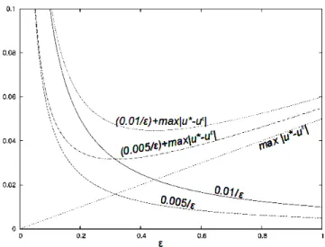
The graph of this total error can be seen in figure 5.2. In this figure, there are two ∆x: 0.01 and 0.005. When ∆xdecreases, the error also decreases for particular ε. It also shows that when ε is big or small, the error increases.

This is approximately similar to the error pattern in figure 5.3a and serves to justify our results.

(34)

Figure 5.2: Estimation from above of the total error for explicit method 2

5.3 Comparisons of solution having different gradient

We are also interested in investigating the choice of ε to get optimal error related to the gradient of the solution near the free boundary point (g_u).

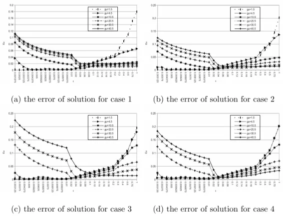
The relation between g_u and the error is shown in (5.14). The gradient of the solution is approximated by calculating the linear regression of five u_i whose values are nearest to the value 0.1. This value is chosen since, based on figure 5.3a-5.3d, when ε = 0.1, they display similar errors for different

∆x.

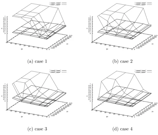
To see the relation between the error of the solutions andg_u, we conduct a few experiments using cases 1-4 with differentg_u. We choose only cases 1-4 since they are enough to represent different kinds of solutions. We set the gradient of the solution at time τ = 7 to be 1 to 40. The results are shown in figures 5.5 and 5.6. Figure 5.5 shows that the range of optimal ε becomes larger wheng_u increases. In addition, the figure 5.6 shows that there are two surfaces. The lower surfaces describe the lower bound of the range for the optimal ε. While the upper surfaces describe the upper bound of the range

(35)

(a)E_u case 1 at time levelτ=9 (b) E_u case 2 at time level τ=9

(c) Eu case 3 at time level τ=9 (d) Eu case 4 at time level τ=9

(e) E_u case 5 at time level τ=9 (f)E_u case 6 at time level τ=7 Figure 5.3: The errors of explicit method 2 for cases 1-6

(36)

(a) E_l case 1 at time level τ=9 (b)E_l case 2 at time levelτ=9

(c)El case 3 at time level τ=9 (d)El case 4 at time levelτ=9

(e)E_l case 5 at time level τ=9 (f)E_l case 6 at time level τ=7 Figure 5.4: The errors of free boundary point of cases 1-6

(37)

figure 5.7. In this figure, each vertical line indicates the range of constant C which applies for the gradient 1 to 40 using specific ∆x. It shows when the constant C is between 0.15-0.16, it satisfies for all cases and ∆x. Therefore, we conclude that the constant C is approximately 0.15-0.16.

(a) the error of solution for case 1 (b) the error of solution for case 2

(c) the error of solution for case 3 (d) the error of solution for case 4 Figure 5.5: The errors of solution for case 1-4 with different gradient with

∆x= 0.000625

(38)

0 0.001 0.002 0.003 0.004 0.005 0.006 0.007 0.008 0.009 0.01 5 0

15 10 25 20 35 30 45 40 0 0.1 0.2 0.3 0.4 0.5 0.6 0.7 0.8 0.9 1

ε

"./case1_lower"

"./case1_upper"

∆x

gu ε

(a) case 1

0 0.001 0.002 0.003 0.004 0.005 0.006 0.007 0.008 0.009 0.01 5 0

15 10 25 20 35 30 45 40 0 0.1 0.2 0.3 0.4 0.5 0.6 0.7 0.8 0.9 1

ε

"./case2_lower"

"./case2_upper"

∆x

gu ε

(b) case 2

0 0.001 0.002 0.003 0.004 0.005 0.006 0.007 0.008 0.009 0.01 5 0

15 10 25 20 35 30 45 40 0 0.1 0.2 0.3 0.4 0.5 0.6 0.7 0.8 0.9 1

ε

"./case3_lower"

"./case3_upper"

∆x

gu ε

(c) case 3

0 0.001 0.002 0.003 0.004 0.005 0.006 0.007 0.008 0.009 0.01 5 0

15 10 25 20 35 30 45 40 0 0.1 0.2 0.3 0.4 0.5 0.6 0.7 0.8 0.9 1

ε

"./case4_lower"

"./case4_upper"

∆x

gu ε

(d) case 4

Figure 5.6: the lower and upper bound of optimalε for cases 1-4

(39)

Figure 5.7: The range of constant C for cases 1-4 with different ∆x

5.4 Comparisons of smoothing characteristic functions

In this experiment, we compare two smoothed characteristic functions. In particular, (5.3) and

(χ^ε)⁰(u) =









 hu

a 0< u < a,

h a≤u≤ε−a,

h(ε−u)

a ε−a≤u≤ε,

0 otherwise,

(5.17)

where

a= ε

b, h= 1

ε−a,

b is a positive number. Function (5.17) has a smoother transition than (5.3).

We want to know whether smooth transitions influence the accuracy. The goal of this experiment is to get the appropriate smoothed characteristic function.

We apply these two functions in equation (1.4) with parameters Q² = 1, Ω = [0,15], a= 1, ∆x= 0.005, and ∆t= 0.9∆x and solve using explicit

(40)

method 2. The errors of each cases at time level τ = 9 (case 6 uses τ = 7) are shown in figure 5.8. The errors are calculated by

E˜_u = max

i=0,...,N k=0,...,M

|u^∗_i(x_i, t_k)−(u^(5.3))^k_i| or E˜_u = max

i=0,...,N k=0,...,M

|u^∗_i(x_i, t_k)−(u^(5.17))^k_i|, (5.18) where u^(5.3) and u^(5.17) are solutions with smoothed characteristic function (5.3) and (5.17) respectively. In this figure, we can see that the errors of solutions using smoothed characteristic function (5.3) and (5.17) for cases 1-6 are relatively same with an order of 10⁻³−10⁻⁴. Therefore, (5.3) is an adequate smoothed characteristic function.

Figure 5.8: Comparison of smoothed characteristic functions

5.5 Comparisons of numerical methods

To compare numerical methods, we conduct two experiments. The first experiment is to numerically solve (5.7) and compare the results with the exact solution (5.10). In order to do this, we consider a case similar to case 1 with