A Self-Adjusting Approach to Identify Hotspots

A Self‑Adjusting Approach to Identify Hotspots

著者 Haoying Han, Xianfan Shu

journal or

publication title

International Review for Spatial Planning and Sustainable Development

volume 5

number 2

page range 104‑112

year 2017‑04‑15

URL http://hdl.handle.net/2297/47859

doi: 10.14246/irspsd.5.2_104

104

ISSN: 2187-3666 (online)

DOI: http://dx.doi.org/10.14246/irspsd.5.2_104

Copyright@SPSD Press from 2010, SPSD Press, Kanazawa

A Self-Adjusting Approach to Identify Hotspots

Haoying Han

and Xianfan Shu

1 Department of Regional and Urban Planning, College of Civil Engineering and Architecture, Zhejiang University

2 Department of Land Management, School of Public Affairs ,Zhejiang University

* Corresponding Author, Email: [email protected] Received: Oct 25, 2016; Accepted: Feb 05, 2017

Key words: Hotspot Detection, Self-adjusting Approach, Clustering, DBSCAN

Abstract: Hotspot identification or detection has been widely used in many fields;

however the traditional grid-based approaches may incur some problems when dealing with point database. This article expands on three types of mismatch problems in grid-based approach and suggests a point-based approach may be more suitable. Inspired by the DBSCAN algorithm, a self-adjusting approach is then proposed for hotspot detection which overcomes the weakness of parameter sensitivity shared by most clustering approaches. Finally, the data of commercial points of interest of a city is used for demonstration.

1. INTRODUCTION

Spatial hotspot identification or detection of point event data has been widely accepted as an integral part of exploratory spatial data analysis (ESDA) across the fields of ecology (Nelson & Boots, 2008), health (Osei &

Duker, 2008; Jeefoo, Tripathi, & Souris, 2010), transportation (Anderson, 2007) and crime (Ratcliffe & McCullagh, 1999; Grubesic, 2006). Hotspot detection provides the foundation for further research on how these hotspots came to being or exert influence, which may help to bring about further scientific or policy implications. It can be concluded that the concept of hotspot is a success considering the number of situations it applies to.

However, a successful concept often means a stretched concept (Sartori, 1984; van Meeteren et al., 2016), that is to say, along with the widespread adoption of hotspot detection is the fuzziness and polyvalence of the underlying concept of ‘hotspot’ itself. Osei and Duker (2008) give an intuitive definition that regards hotspot as a condition indicating some form of clustering in a spatial distribution. Lawson (2010) uses the item “unusual aggregation” of events to define a clustering of a spatially-referenced featured and summarizes that intensity, spatial integrity, size and shape are usually used as the criteria to determine whether an aggregation of events can be considered ‘unusual’ . Nevertheless, there still needs local knowledge or prior knowledge to specify these criteria.

After reviewing indicators for assessing local spatial association and

putting forward a new one, Anselin (1995) argues local spatial clusters,

Han & Shu 105 sometimes referred to as hot spots, can be identified as those locations or sets of contiguous locations with statistically significant local spatial associations. This definition follows the maxim ‘let the data speak for themselves’ (Gould, 1981) and provides another perspective to define

‘hotspot’ which focuses on the features of spatial elements rather than their aggregations as the intuitive definition does.

In fact these two perspectives represent two different epistemologies about hotspot. The former one considers hotspot as a special cluster of spatial elements, while the latter considers it as a cluster of special spatial elements. Such a difference inevitably brings about different methodological axes along which the approaches of hotspot detection develop. However, many of these approaches are grid-based (Yu, W. et al., 2016), which may incur some mismatching problems when dealing with point event data.

In next section, we will expand on the underlying mismatch problems of employing grid-based approach to detect hotspots of point event data. To overcome these problems, we will propose a modified version of density based spatial clustering of application with noise (DBSCAN). This is followed by an empirical example using commercial POIs (point of interest) data of Xiaoshan, Hangzhou to detect commercial hotspots there. The article ends with conclusions and suggestions for further work.

2. DRAWBACKS OF GRID-BASED APPROACH 2.1 Scale mismatch

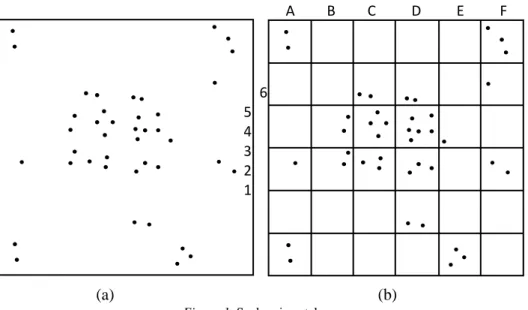
The first mismatch is about the scale of grid. Fig1 (a) indicates a case where a hotspot （in the middle of the grid） is bundled with discrete non- hotspot points in an oversized grid. If this grid is identified as a (part of) hotspot, there will be an ‘over-detecting’ problem because it involves some non-hotspot points. Similarly, a non-hotspot consequence of identification denotes an ‘under-detecting’ problem because actually there is a neglected local hotspot in this grid. So oversize means problem anyhow.

(a) (b)

Figure 1. Scale mismatch

In an undersized case showed in Fig 1(b), a problem of either over- detecting or under-detecting is also unavoidable. In an undersized grid system, a hotspot will be divided into too many parts to make themselves distinguishable (like C-2 versus A-1 in Fig 1(b)). So again this hotspot is

6 5 4 3 2 1

bundled with non-hotspot points, and the case goes similarly with the oversized situation. A solution is to introduce more detecting criteria such as size or spatial integrity, but this will largely perplex the process of parameter calibration.

2.2 Shape mismatch

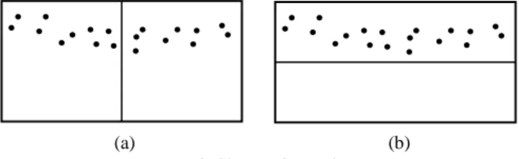
The shape mismatch occurs when the grid shape can’t correspond with those of hotspots well enough to make them detectable. Fig 2(a) illustrates the difficulty for a square-grid system to detect a linear hotspot. However, linear hotspots are actually quite common such as plants along rivers, polluted air along wind, and shops along streets.

(a) (b) Figure 2. Shape mismatch

2.3 Location mismatch

Even eventually we manage to pick out the most proper grid scale and shape, there is still another thorny problem concerning the locations of grids.

Figure3 illustrates a case of detection failure resulted from location mismatch where a same hotspot of point events is divided by two grid systems with the same scale and shape but different spatial distributions respectively. It is obvious that Figure 3(a) is the situation where detection failure occurs more probably, because the aggregation pattern of this hotspot is “diluted” by four grids here and each grid may be unable to reach the intensity threshold. Yet a slight shift to the grid system in Figure 3(b) makes this hotspot detectable.

Besides, compared with scale mismatch, location mismatch is more locally problematic. This means a solution’s validity is always localized; that is to say, a modification in one place may lead to a new mismatch problem elsewhere, so it’s almost impossible to find a globally suitable solution.

(a) (b)

Figure 3. Location mismatch

Han & Shu 107

3. OUR APPROACH 3.1 DBSCAN: pros and cons

Theoretically speaking, in hotspot detection for point event data, gridding process is something like feature extraction in dimension reduction -- usually we establish a feature to measure the aggregation degree at a lower spatial resolution with a cost of losing the information of every point’s precise location. How this feature is established or extracted determines how much information we will actually lose, and all of the three types of mismatch can be attributed to the information loss caused by gridding process.

Consequently an approach which clusters the original point event data directly may help to avoid the mismatch problems above.

Actually, in clustering field there is a history of decades of point-density- based approach since Ester et al. (1996) firstly established an algorithm called DBSCAN (Density Based Spatial Clustering of Applications with Noise), which is one of most common and citied clustering algorithms in scientific literature (Uncu et al., 2006; Chakraborty & Nagwani, 2014).

The DBSCAN algorithm starts with an arbitrary point p in database D, which should have at least MinPts neighbors within a distance of Eps from it. Then p (marked as a core point, otherwise as a border point) and its neighbors are assigned into a new cluster. The same searching process will be done to each neighbor of point p and if this point reaches the core-point threshold, it and its neighbors will be assigned to the former cluster, otherwise it will be marked as a border point and the searching process stops. So finally an iterative process goes on until there are no new points to be assigned. This is repeated until all points in D traversed. It can be established mathematically on the concepts and terms as follows (Ester et al., 1996).

Definition 1: (Eps-neighborhood of a point) The Eps-neighborhood of a point p, denoted by N

(p) , is defined by N

(p) = {q ∈ D|dist(p, q) ≤ Eps} , where D is the database p and q belong to and dist(p, q) is distance between points p and q.

Definition 2: (directly density-reachable) A point p is directly density- reachable from point q wrt. Eps, MinPts if

1) p ∈ N

(q) and 2) |N

(q)| ≥ MinPts .

Definition 3: (density-reachable) A point p is density-reachable from a point wrt. Eps and MinPts if there is a chain of points p

, … p

, p

= q, p

= p such that p

is directly density-reachable from p

.

Definition 4: (density-connected) A point is density-connected to a point q wrt. Eps and MinPts if there is a point o such that both p and q are density- reachable from o wrt. Eps and MinPts.

Definition 5: (cluster) A cluster C wrt. Eps and MinPts is a non-empty subset of D satisfying the following conditions:

1) ∀ p, q: if p ∈ D and q is density-reachable from p wrt. Eps and MinPts, the q ∈ C. (Maximality)

2) ∀ p, q ∈ C: p is density-connected to q wrt. Eps and MinPts.

(Connectivity)

Definition 6: (noise) Let C

, … , C

be the clusters of the database D wrt.

Parameters Eps

and MinPts

, i =1,…k. Then we define the noise as the set

of points in a database D not belonging to any cluster C

, i.e. noise = {p ∈

D| ∀ i: p ∉ p }.

Focusing on point-to-point associations, DBSCAN has the ability to detect clusters of arbitrary shape, making it possible to avoid the shape mismatch in grid-based approach. Because the ‘scanning’ process (searching for neighbors) in DBSCAN is always point-centered, location mismatch is also avoidable. So the shared problem is the calibration of scale (grid size versus Eps) and intensity threshold (usually density versus MinPts).

In fact, one of the main drawbacks of DBSCAN just rests with the fact that its result is highly sensitive to Eps and MinPts (Cai, Xie, & Ma, 2004).

As a result, there emerge a number of studies aiming to propose a self- adjusting calibrating method for Eps and MinPts (Xia & Jing, 2009). Some studies (Feng & Ge, 2004; Yue et al., 2005) partly solve this problem by proposing a self-adjusting approach for one parameter. Uncu et al. (2006) and Mahran and Mahar (2008) both propose a self-adjusting variations of DBSCAN named GRIDBSCAN whose Eps and MinPts can be calculated automatically, but obviously they are also both grid-based, which may result in the mismatch problems mentioned above. Other self-adjusting variations of DBSCAN can be found in the work of Yu, X., Zhou, and Zhou (2005) and Liu, Zhou, and Wu (2007). These two algorithms are both based on a KNN (the kth nearest neighbors) approach, which still lack a mathematic calibration process even it is proved not strictly that the influence of k is not so considerable (Yu, X., Zhou, & Zhou, 2005; Liu, Zhou, & Wu, 2007).

3.2 To a self-adjusting approach

3.2.1 An alternative to MinPts

In DBSCAN, MinPts is set to identify those points around which the density is relatively higher, so the fundamental purpose of calibration of MinPts lies in finding a scientific and ‘natural’ threshold. Here calibration of MinPts is more of a tool rather than a purpose. Consequently, instead of searching for other parameters with less requirement of prior field knowledge to achieve the self-adjusting calibration of MinPts as most previous studies do, a more suitable and convenient way is to find another density indicator which is self-adjusting in itself.

The local indicator of spatial association (LISA) is a promising candidate for such an indicator. Firstly, it follows the maxim “let the data speak for themselves”, which means LISA has an innate purpose to be self-adjusting.

Besides, as defined by Anselin (1995), the LISA gives each observation an indication of the extent of significant spatial clustering of similar values around the observations, and if the “value” of each observation is specified as the neighboring density, correspondingly the LISA can indicate the extent to which points with plenty of neighbors clusters spatially.

The most common LISA is local Moran’ I proposed by Anselin (1995), and for an observation i it is defined as,

𝐼𝐼

=

∑

𝑊𝑊(𝑖𝑖, 𝑗𝑗)(𝑋𝑋

− 𝑋𝑋) (1)

𝑋𝑋 =

(2) S =

(3)

Where 𝐼𝐼

is the local Moran’s index of observation i, 𝑋𝑋

is the feature

value of observation i, 𝑋𝑋 is the mean of 𝑋𝑋

, 𝑁𝑁′ is the number of observations

which has at least one neighbor, 𝑊𝑊(𝑖𝑖, 𝑗𝑗) is the spatial weight between

observation i and j, and for point event data, 𝑊𝑊(𝑖𝑖, 𝑗𝑗) is usually calculated as,

Han & Shu 109

𝑊𝑊(𝑖𝑖, 𝑗𝑗) = � 1, 𝑖𝑖𝑖𝑖 𝑑𝑑𝑖𝑖𝑑𝑑𝑑𝑑(𝑖𝑖, 𝑗𝑗) ≤ 𝐸𝐸𝐸𝐸𝑑𝑑, 𝑖𝑖 ≠ 𝑗𝑗

0, 𝑜𝑜𝑑𝑑ℎ𝑒𝑒𝑒𝑒𝑒𝑒𝑖𝑖𝑑𝑑𝑒𝑒 (4) For ease of interpretation, the weights 𝑊𝑊(𝑖𝑖, 𝑗𝑗) should be in a row- standardized form. As for the value of 𝐼𝐼

, a positive value means i is surrounded by similar observations (‘High value to High values’ or ‘Low value to Low values’), and a negative value means it is surrounded by distinguished observations (‘High value to Low values’ or ‘Low value to High values’). Higher absolute value of 𝐼𝐼

means more significant patterns.

Now we define 𝑋𝑋

as the number of points within a distance of Eps from point I, then 𝐼𝐼

can be used to indicate how the points are spatially clustered.

A positive value of 𝐼𝐼

now indicates two situations, one is where both point i and its neighbors have a plenty of neighbors (‘High value to High values’), the other one is where both point I and its neighbors have few neighbors (‘Low value to Low values’). These two situations can be further classified according to 𝑋𝑋

, the number of neighbors of point I.

Considering DBSCAN’s similar process, we can assign points of the former type as the core point of a hotspot, and the border point can be defined as the points which don’t reach the core point standard. The modified terms and definitions are as follow,

Definition 7: (directly autocorrelation-reachable) A point p is directly autocorrelation-reachable from point q wrt. Eps if

1) p ∈ N

(q)

2) �N

(q)� >

∑

|N

(i)| and 3) I(q) > 0

Definition 8: (autocorrelation-reachable) A point p is autocorrelation - reachable from a point wrt. Eps if there is a chain of points p

, … p

, p

= q, p

= p such that p

is directly density-reachable from p

.

Definition 9: (autocorrelation-connected) A point is density-connected to a point q wrt. Eps if there is a point o such that both p and q are density- reachable from o wrt. Eps

Definition 10: (hotspot) A hotspot H wrt. Eps is a non-empty subset of D satisfying the following conditions:

1) ∀ p, q: if p ∈ D and q is density-reachable from p wrt. Eps, the q ∈ H.

(Maximality)

2) ∀ p, q ∈ H: p is density-connected to q wrt. Eps. (Connectivity)

Definition 11: (autocorrelation noise) Let H

, … , H

be the clusters of the database D wrt. Eps

, i =1,…k. Then we define the noise as the set of points in a database D not belonging to any cluster H

, i.e. noise = {p ∈ D| ∀ i: p ∉ p }.

3.2.2 Calibration of Eps

For a clustering algorithm, the optimal clustering result can be achieved by analyzing validity index, and at the same time the inputted parameters can also be adaptively adjusted (Feng & Ge, 2004). Here the most common validity index, DB index is employed to calibrate the parameter Eps. DB index is defined as follows (Davies & Bouldin, 1979),

𝑅𝑅 =

∑

𝑅𝑅

𝑖𝑖=1

(5) 𝑅𝑅

= max

𝑖𝑖≠𝑗𝑗

𝑅𝑅

(6) 𝑅𝑅

=

𝑖𝑖𝑗𝑗

(7) 𝑆𝑆

= �

𝑖𝑖

∑

|𝑋𝑋

− 𝐴𝐴

|

�

(8)

𝑀𝑀

= �∑

|𝑎𝑎

− 𝑎𝑎

|

�

(9) where 𝑅𝑅 is the DB index, N is the number of clusters, 𝑅𝑅

is a similarity indicator between cluster i and j; 𝑆𝑆

measures the dispersion of cluster i, 𝑇𝑇

is the number of observations belonging to cluster i, 𝑋𝑋

is the feature vector of observation j, and 𝐴𝐴

is the centered feature vector of cluster i; 𝑀𝑀

measures the distance between clusters i and j, n is the number of features, 𝐴𝐴

and 𝑎𝑎

are the centered feature vector of cluster i and j respectively. P and q are both distance parameters, normally equaling to 2 to derive Euclidean distances. In general, a lower value of DB index means better performance of the clustering algorithm.

In our approach, there are three “clusters”, core points, border points and noise, so N equals 3. The number of neighbors wrt. Eps is the only feature for each point, so n equals 1. Eps is determined when DB index achieves minimum.

4. EXPERIMENTAL RESULTS

In this section, the proposed approach is applied to detect the commercial hotspot in Xiaoshan District, Hangzhou. The database consists of 15432 POIs (points of interest) of shopping and food, which were collected from DaZhongDianPing by the end of 2015.

Figure 4 illustrates how DB index changes as Eps increases from 50m to 1000m by a step of 50m. Obviously, DB index achieves minimum when Eps is at 400 (m), therefore Eps is calibrated at 400. Figure 5 illustrates the detection result of the commercial hotspots in Xiaoshan. The magnified view focusing on the downtown area of Xiaoshan shows us our approach inherits the ability to detect clusters with arbitrary shape from DBSCAN algorithm.

Figure 4. DB – Eps relation

0 1 2 3 4 5

0 200 400 600 800 1000 1200

DB Index

Eps (meter)

Han & Shu 111

Figure 5. Commercial hotspots in Xiaoshan

5. CONCLUSIONS AND DISCUSSION

Hotspot detection is often one of the first steps in the analysis of spatial data. Considering the inherent drawbacks of grid-based approach to detect hotspots for point event data, we propose a point-based approach inspired by DBSCAN algorithm. A local indicator for spatial autocorrelation and a clustering validity index are integrated into this approach to achieve self- adjusting parameter calibration. An empirical example is presented to show this approach’s applicability.

Following the maxim ‘let the data speak for themselves’, our approach does help to minimize the possible human intervention which may incur mistaken detection results in hotspot detection, making it possible for comparing detection results among different regions. This does not mean, however, there is no need of prior knowledge in hotspot detection. Actually, in some fields, the performance of detection results depends a lot on prior knowledge; e.g., if we do not know well enough about which level of visitor flowrate may lead to stampede, any hotspot detection for visitors will lose its validity because of the hidden danger.

There is also much work to do to refine this approach. For example, more work is needed to accelerate the calibration of Eps and the selection of clustering validity index also deserves discussions. Theoretic efforts are needed to explore the relationship between clustering and hotspot detection.

REFERENCES

Anderson, T. (2007). "Comparison of Spatial Methods for Measuring Road Accident

‘Hotspots’: A Case Study of London". Journal of Maps, 3(1), 55-63.

Anselin, L. (1995). "Local Indicators of Spatial Association—Lisa". Geographical analysis, 27(2), 93-115.

Cai, Y., Xie, K., & Ma, X. (2004). "An Improved Dbscan Algorithm Which Is Insensitive to Input Parameters". Acta Scicentiarum Naturalum Universitis Pekinesis, 40(3), 480-486.

Chakraborty, S., & Nagwani, N. K. (2014). "Analysis and Study of Incremental Dbscan Clustering Algorithm". arXiv preprint arXiv:1406.4754.

Davies, D. L., & Bouldin, D. W. (1979). "A Cluster Separation Measure". IEEE Transactions on Pattern Analysis and Machine Intelligence, (2), 224-227.

Ester, M., Kriegel, H.-P., Sander, J., & Xu, X. (1996). "A Density-Based Algorithm for Discovering Clusters in Large Spatial Databases with Noise". Kdd, 96(34), 226-231.

Feng, P., & Ge, L. (2004). "Adaptive Dbscan-Based Algorithm for Constellation Reconstruction and Modulation Identification". Proceedings of Radio Science Conference, Beijing, pp. 177-180.

Gould, P. (1981). "Letting the Data Speak for Themselves". Annals of the Association of American Geographers, 71(2), 166-176.

Grubesic, T. H. (2006). "On the Application of Fuzzy Clustering for Crime Hot Spot Detection". Journal of Quantitative Criminology, 22(1), 77-105.

Jeefoo, P., Tripathi, N. K., & Souris, M. (2010). "Spatio-Temporal Diffusion Pattern and Hotspot Detection of Dengue in Chachoengsao Province, Thailand". International journal of environmental research and public health, 8(1), 51-74.

Lawson, A. B. (2010). "Hotspot Detection and Clustering: Ways and Means". Environmental and Ecological Statistics, 17(2), 231-245.

Liu, P., Zhou, D., & Wu, N. (2007). "Vdbscan: Varied Density Based Spatial Clustering of Applications with Noise". Proceedings of Service Systems and Service Management, pp.

1-4.

Mahran, S., & Mahar, K. (2008). "Using Grid for Accelerating Density-Based Clustering".

Proceedings of Computer and Information Technology, pp. 35-40.

Nelson, T. A., & Boots, B. (2008). "Detecting Spatial Hot Spots in Landscape Ecology".

Ecography, 31(5), 556-566.

Osei, F. B., & Duker, A. A. (2008). "Spatial and Demographic Patterns of Cholera in Ashanti Region-Ghana". International Journal of Health Geographics, 7(1), 44.

Ratcliffe, J. H., & McCullagh, M. J. (1999). "Hotbeds of Crime and the Search for Spatial Accuracy". Journal of Geographical Systems, 1(4), 385-398.

Sartori, G. (1984). "Guidelines for Concept Analysis". In Collier, D. & Gerring, J. (Eds.), Social Science Concepts: A Systematic Analysis (pp. 97–151). New York/London:

Routledge.

Uncu, O., Gruver, W. A., Kotak, D. B., Sabaz, D., Alibhai, Z., & Ng, C. (2006). "Gridbscan:

Grid Density-Based Spatial Clustering of Applications with Noise". Proceedings of Systems, Man and Cybernetics, pp. 2976-2981.

van Meeteren, M., Poorthuis, A., Derudder, B., & Witlox, F. (2016). "Pacifying Babel’s Tower: A Scientometric Analysis of Polycentricity in Urban Research". Urban Studies, 53(6), 1278-1298.

Xia, L.-N., & Jing, J.-W. (2009). "Sa-Dbscan: A Self-Adaptive Density-Based Clustering Algorithm". Journal of the Graduate School of the Chinese Academy of Sciences, 26(4), 530-538.

Yu, W., Ai, T., Yang, M., & Liu, J. (2016). "Detecting "Hot Spots" of Facility Pois Based on Kernel Density Estimation and Spatial Autocorrelation Technique". Geomatics and Information Science of Wuhan University, 41(2), 222-227.

Yu, X., Zhou, D., & Zhou, Y. (2005). "A New Clustering Algorithm Based on Distance and Density". Proceedings of Services Systems and Services Management, pp. 1016-1021.

Yue, S.-H., Li, P., Guo, J.-D., & Zhou, S.-G. (2005). "A Statistical Information-Based Clustering Approach in Distance Space". Journal of Zhejiang University-Science A, 6A(1), 71-78.