Mechanism design without quasilinearity
T omoya K azumura
Department of Industrial Engineering and Economics, Tokyo Institute of Technology
D ebasis M ishra
Economics and Planning Unit, Indian Statistical Institution
S higehiro S erizawa
Institute of Social and Economic Research, Osaka University
This paper studies a model of mechanism design with transfers where agents’
preferences need not be quasilinear. In such a model, (i) we characterize domi- nant strategy incentive compatible mechanisms using a monotonicity property, (ii) we establish a revenue uniqueness result (for every dominant strategy imple- mentable allocation rule, there is a unique payment rule that can implement it), and (iii) we show that every dominant strategy incentive compatible, individually rational, and revenue-maximizing mechanism must charge zero payment for the worst alternative (outside option). These results are applicable in a wide variety of problems (single object auction, multiple object auction, public good provision, etc.) under suitable richness of type space. In particular, our results are applica- ble to two important type spaces: (a) type space containing an arbitrarily small perturbation of quasilinear type space and (b) type space containing all positive income effect preferences.
Keywords. Incentive compatibility, individual rationality, monotonicity, non- quasilinear preferences, revenue equivalence.
JEL classification. D82, D44, D40.
1. Introduction
We analyze a model of mechanism design with transfers where preferences of agents over transfers are not necessarily quasilinear. We assume agents have classical prefer- ences over the set of consumption bundles, where a consumption bundle consists of an alternative and a transfer amount. A preference (type) is classical if it is monotone and continuous in transfers.
Tomoya Kazumura: [email protected] Debasis Mishra: [email protected]
Shigehiro Serizawa: [email protected]
We are grateful to the two anonymous referees for their insightful comments. We also thank Sushil Bikhchandani, Juan Carlos Carbajal, James Schummer, participants at numerous conferences, and, in par- ticular, Arunava Sen, for useful comments. We gratefully acknowledge financial support from the Joint Usage/Research Center at ISER, Osaka University and the Japan Society for the Promotion of Science (Kazu- mura, 14J05972; Serizawa, 15J01287, 15H03328, 15H05728). Debasis Mishra acknowledges the hospitality and support of ISER, Osaka University.
©
2020 The Authors. Licensed under the
Creative Commons Attribution-NonCommercial License 4.0.Available at
https://econtheory.org.https://doi.org/10.3982/TE2910We provide results that cover a variety of important problems: the single object auc- tion problem, the multi-object auction problem, the public good provision problem, and so on. If the type space satisfies a richness property, we provide a simple mono- tonicity condition that along with a posted-price property, is necessary and sufficient for a mechanism to be (dominant strategy) incentive compatible. The posted-price prop- erty requires the payment decisions at various types to agree whenever the allocation decisions at these types agree. Further, we establish a revenue uniqueness result: for every implementable allocation rule, there is a unique payment rule such that the cor- responding mechanism is incentive compatible. Though we do not have revenue equiv- alence in our model, our results can be interpreted as a counterpart of the monotonicity and revenue equivalence results with quasilinearity.
There are at least two important type spaces where our results apply. Let Q be the set of all quasilinear preferences in some standard problem. The first example of a type space where our results apply is any superset of Q containing “small perturbations” of types in Q . Our second example is a type space containing all positive income effect preferences.
We study the implications of individual rationality without quasilinearity. Recall that a straightforward consequence of revenue equivalence in a quasilinear environment is that a revenue-maximizing, incentive compatible, and individually rational mechanism charges zero payment for allocating the worst alternative. In other words, individual rationality “binds” for the worst alternative. We show that this result continues to remain valid in arbitrary non-quasilinear type spaces.
We apply our results to provide a template for identifying an optimal contract in a principal–agent model. An important insight from the mechanism design literature with quasilinearity is that the optimization problem for finding an optimal contract can be reduced to an optimization problem over the set of monotone allocation rules. The objective function can be rewritten in terms of the allocation rule using the revenue equivalence formula. Furthermore, the incentive and individual rationality constraints can be replaced by a monotonicity constraint on the allocation rule. This approach is key to solving tractable optimal contract problems (Mussa and Rosen 1978, Myerson 1981). We show that this approach can be extended to our model with non-quasilinear preferences. We now proceed to the details.
2. T he model
Let A be a finite set of alternatives with | A | ≥ 2. We endow A with a strict partial or-
der . This partial order reflects a possible ex ante ordering of alternatives if there is
no monetary compensation. The partial order may be empty; for instance, if A is the
set of public goods and there is no ex ante distinction among the public goods. In the
problem of selling multiple units of a homogeneous good, a standard assumption is that
more units are preferred to less. If there are two alternatives a and b with a being k units
of the good and b being units of the good, we may impose a b if and only if k > . In
combinatorial auctions for selling multiple objects, may be the partial order induced
by the set inclusion relation over subsets of objects.
There is a single agent in our model. Our main results extend to a model with mul- tiple agents in a straightforward manner as our solution concept is dominant strat- egy equilibrium. We allow for monetary transfers or payments. Hence, a consump- tion bundle for the agent is a pair (a p), where a ∈ A is an alternative and p ∈ R is the payment of the agent. The set of all such consumption bundles is denoted by Z := { (a p) : a ∈ A p ∈ R} .
The agent has a complete and transitive preference over Z . A typical preference is denoted by R with its strict and indifferent components denoted by P and I , respectively.
We call a preference R over Z classical if it satisfies the following conditions.
• Money monotonicity. For all p p
∈ R with p > p
and for all a ∈ A, (a p
)P(a p).
• Respect for . For all p ∈ R and for all a b ∈ A with a b, (a p)P(b p).
• Continuity. For all z ∈ Z , the sets { z
∈ Z : zRz
} and { z
∈ Z : z
Rz } are closed.
• Possibility of compensation. For every z ∈ Z and for every a ∈ A, there exists p and p
such that (a p)Rz and zR(a p
).
While monotonicity and continuity are natural restrictions, we impose the possibil- ity of a compensation condition for technical reasons. We are only concerned with clas- sical preferences in this paper, so whenever we write “preference,” we mean a classical preference.
2.1 Indifference vectors
It is convenient to think of a preference in terms of its indifference vectors. A vector v ∈ R
|A|is an indifference vector of preference R if for all a b ∈ A, we have (a v
a)I(b v
b).
Denote the set of all indifference vectors of R by I (R). For every preference, its indif- ference vectors satisfy many natural properties. So as to discuss them, we introduce the notion of a valuation.
The valuation of the agent with preference R for alternative a at consumption bun- dle z is denoted by V
R(a z), where (a V
R(a z))Iz. In other words, V
R(a z) is the unique payment that makes the agent indifferent between consumption bundle z and (a V
R(a z)). The existence of V
R(a z) and its uniqueness is guaranteed by the assump- tions on preferences. As a result, for every preference R and for every pair of distinct indifference vectors v v
∈ I (R), we have either v > v
or v
> v, i.e., v and v
do not in- tersect.
1Further, every indifference vector of R respects : for every v ∈ I (R), we have v
a> v
bif a b.
A typical indifference vector v of a preference R can be represented by the diagram shown in Figure 1. We use such figures throughout our paper and we refer to them as indifference diagrams.
2Figure 1 shows how a indifference diagram can be constructed for four alternatives. Each horizontal line in the indifference diagram corresponds to a
1
Whenever, we write
v > v, we mean
vx> vxfor all
x∈A.2
William Thomson popularized such diagrams to represent preferences in private goods models with
indivisible goods and money.
Figure 1. An indifference vector for the case a b c d.
Figure 2. A preference and its indifference diagram for the case a b c d.
unique alternative. Every point on a horizontal line corresponds to a payment level. So the four horizontal lines in this indifference diagram comprise the set of all consump- tion bundles Z . As we move rightward along a horizontal line, the payment of the agent increases. Hence, consumption bundles to the right (left) of the indifference vector v in Figure 1 are worse (respectively, better) than the four consumption bundles correspond- ing to v.
An equivalent way to think of a preference R is through its infinite set of indifference vectors I (R). Hence, the indifference diagram of a preference consists of an infinite collection of such vectors; a representative indifference diagram is shown in Figure 2.
2.2 Positive income effect
Two special kinds of preferences are worth highlighting. Vectors v v
∈ R
|A|are parallel if for all a b ∈ A, we have v
a− v
b= v
a− v
b. Vectors v v
∈ R
|A|with v > v
satisfy decreasing differences (DD) if for all a b ∈ A, we have
[ v
a> v
b] ⇒
v
a− v
b> v
a− v
bFigure 3. Indifference diagram of a preference satisfying PIE.
F igure 4. Indifference diagram of a preference that does not satisfy PIE.
D efinition 1. A preference R is quasilinear if every pair of indifference vectors v v
∈ I (R) is parallel. A preference R satisfies positive income effect (PIE) if every pair of indif- ference vectors v v
∈ I (R) satisfies DD.
We denote the set of all quasilinear preferences and the set of all preferences sat- isfying PIE by Q and R
+, respectively.
3Note that Q ∩ R
+= ∅. For any R ∈ R
+, the indifference diagram corresponding to R is shown in Figure 3.
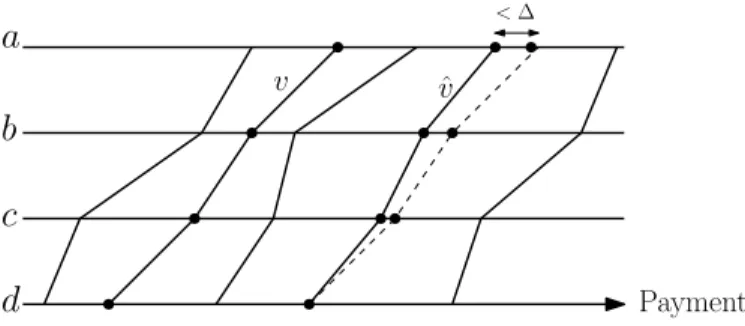
To understand PIE, take any R ∈ R
+and v ∈ I (R). Consider another vector v ˆ defined by v ˆ
x= v
x− δ ∀ x ∈ A, where δ > 0. Suppose that for some a ∈ A, we have v
a> v
xfor all x = a (as in Figure 3). Then we see that for any x = a, the consumption bundle (a v ˆ
a) is strictly preferred to (x v ˆ
x) according to R. As we decrease the payment by a constant amount δ from v to v ˆ (i.e., increase the wealth level by δ), the highest payment consump- tion bundle at v is now the most preferred. This is the idea of a positive income effect, which is usually observed in normal goods. Contrast this with a quasilinear preference, where the agent will be indifferent between all the bundles on v. ˆ
The decreasing differences property imposes restrictions on admissible indifference vectors. To further highlight these restrictions, consider A = { a b } and that is empty.
The indifference diagram for a preference R for this example is shown in Figure 4. We
3
To be precise,
Qis the set of all preferences that respect and are quasilinear. For notational simplicity,
we suppress the dependence of
Qon . Further, we refer to
Qas
thequasilinear domain, meaning the
quasilinear domain corresponding to a given
. A similar comment applies toR+and other domains
discussed henceforth.
argue that R does not satisfy PIE. This is because the indifference vectors v v
∈ I (R) satisfy v > v
but fail DD: v
b> v
abut v
b− v
a< 0 < v
b− v
a. This is the intuition for Fact 1 below.
4F act 1 (Remark 2 in Zhou and Serizawa (2018)). Suppose R is a preference that satisfies PIE. Then there exists a weak ordering on the set of alternatives such that for every a b ∈ A and every v ∈ I (R),
[ a b ] ⇒ [ v
a≥ v
b]
Fact 1 implies that even if is empty, there is an underlying weak order for every positive income effect preference. Notice that, potentially, such a weak order may be different for different positive income effect preferences. To understand the interaction between and , fix an R that satisfies PIE. Then (a) is weak but complete (but may be empty); (b) must match whenever the latter is nonempty, i.e., for any a b ∈ A, a b implies a b holds but b a does not hold. Hence, if is a complete order, = . We are also concerned with the following weaker notion of decreasing differences.
A pair of vectors v v
∈ R
|A|with v > v
satisfies decreasing differences ( DD) if for all a b ∈ A, we have
[ a b ] ⇒
v
a− v
b> v
a− v
bIf v, v
respect and satisfy DD, they satisfy DD. Based on this, we can define a weaker notion of PIE. A preference R satisfies positive income effect ( PIE) if every pair of indifference vectors v v
∈ I (R) satisfies DD. Let R
+denote the set of all preferences satisfying PIE. Obviously, R
+⊆ R
+for each . If is complete and v respects , then a b if and only if v
a> v
b. Hence, R
+= R
+if is complete. This equivalence is not necessarily true if is not complete. For instance, the preference shown in Figure 4 satisfies PIE vacuously since is empty (though it does not satisfy PIE).
2.3 Domains, mechanisms and questions
Let R be the set of all (classical) preferences. A type space or domain D is any subset of R . A mechanism on a domain D is a pair of maps (f p), where f : D → A is an allocation rule and p : D → R is a payment rule. Throughout the paper, we consider only allocation rules that are onto: for every a ∈ A, there exists some preference R ∈ D such that f (R) = a.
5We investigate the implications of two desiderata for our mechanisms.
Definition 2. A mechanism (f p) on D is dominant strategy incentive compatible (DSIC) if for every R R
∈ D , we have (f (R) p(R))R(f (R
) p(R
)).
In addition to incentive compatibility, we consider individual rationality. Whenever we talk about individual rationality, we assume the existence of an alternative a
0∈ A
4
Its proof is available in Appendix A of
Zhou and Serizawa(2018).
5
In some sense, “ontoness” is without loss of generality. If we have an allocation rule
fwhose range is
AA, then we can consider the entire model whereAis replaced by
A.
such that a a
0for all a = a
0. Alternative a
0can be interpreted as the outside option, for instance, not getting any object in a multiple object auction model or not providing any public good in a public good model. We do not require the existence of such an alternative for our results involving only DSIC.
D efinition 3. A mechanism (f p) on D satisfies individual rationality (IR) if for every R ∈ D , we have (f (R) p(R))R(a
00).
We answer three questions in our model of preferences.
• In the quasilinear domain, a monotonicity condition of allocation rule and a rev- enue equivalence formula characterize a DSIC mechanism. What is the analogue of such a characterization without quasilinearity?
• What happens to revenue equivalence without quasilinearity?
• Does the IR constraint bind for the worst alternative without quasilinearity?
3. R ichness
Our results require our domains to be suitably rich. The weakest richness condition that we require is the following.
D efinition 4. A domain of preferences D satisfies one-point (OP) richness if for every v ∈ R
|A|that respects , there exists R ∈ D such that v ∈ I (R).
OP richness is satisfied by Q , the set of all quasilinear preferences. It is therefore sat- isfied by any domain D ⊇ Q . It is also satisfied by R
+, the set of all positive income effect preferences (and supersets of that). OP richness allows us to construct a preference that has one specific indifference vector. It is silent on the other indifference vectors in the preference.
The quasilinear domain Q satisfies OP richness. By definition, Q contains all quasi- linear preferences respecting . OP richness is violated if we take a strict subset of Q . For example, suppose A = { a
0a
1a
2} with a
2a
1a
0. A quasilinear preference is rep- resented by a valuation vector v ∈ R
3+with v
a2> v
a1> v
a0= 0. The quasilinear domain Q contains preferences corresponding to all such vectors in R
3+. Now consider a spe- cific kind of quasilinear preference whose valuation vector is v
a2= 2θ, v
a1= θ, v
a0= 0 for some θ ∈ R
++. The set of all such preferences is
Q
1:=
R ∈ Q : ∃ θ ∈ R
++such that V
Ra
1(a
00)
= θ V
Ra
2(a
00)
= 2θ It is clear that Q
1is a strict subset of Q and it contains very specific “one-dimensional”
quasilinear preferences. The domain Q
1fails OP richness. Though our richness condi- tions exclude domains like Q
1, they still admit interesting domains where a large class of DSIC mechanisms exist. For instance, the family of Groves mechanisms are DSIC in Q .
Our next notion of richness requires the existence of a preference for some specific
pair of indifference vectors.
Figure 5. Indifference diagram of a candidate preference for satisfying TP
+richness.
D efinition 5. Let > 0. Vectors v, v ˆ with v > v ˆ are
+parallel if (i) they satisfy DD and (ii) | ( v ˆ
a− ˆ v
b) − (v
a− v
b) | < for all a b ∈ A.
Our next richness condition gives us the flexibility to construct some preference us- ing every pair of
+parallel vectors.
D efinition 6. Let > 0. A domain D satisfies
+two-point richness (TP
+richness) if for every v, v ˆ with v > v ˆ such that v, v ˆ are
+parallel and v, v ˆ respect , there exists R ∈ D such that v v ˆ ∈ I (R).
Notice that TP
+richness is for a fixed . Obviously, if we choose
> and D sat- isfies TP
+richness, it also satisfies TP
+richness. Next, TP
+richness is about existence of some R ∈ D for every pair v, v ˆ satisfying the two conditions in the definition above.
This preference may be different for a different pair of vectors. Further, the richness condition is silent about the properties of other indifference vectors in this preference.
For illustration, consider the indifference diagram in Figure 5. The indifference diagram shows two indifference vectors v and v ˆ that are
+parallel and respect . The vectors v and the one represented by dashed lines are parallel. It also shows a preference R (show- ing a subset of indifference vectors of R) such that v v ˆ ∈ I (R). Notice that there are other indifference vectors of R that are not necessarily
+parallel. For this reason, a domain satisfying TP
+richness need not contain the quasilinear domain. Example 1, which is given later in this section, highlights this point.
We now introduce our final notion of richness.
D efinition 7. Let > 0. Vectors v, v ˆ with v > v ˆ are
parallel if (i) they satisfy DD and (ii) | ( v ˆ
a− ˆ v
b) − (v
a− v
b) | < for all a b ∈ A.
Notice that
parallel requires a pair of vectors to satisfy DD but
+parallel re-
quires them to satisfy DD. If v, v ˆ satisfy decreasing differences, the first condition in
Definition 7 is automatically satisfied. Hence, any pair of vectors v, v ˆ that are
+parallel
are also
parallel. Further, if is a complete order, for every vector v that respects ,
we have a b if and only if v
a> v
b. Hence, if is complete, a pair of vectors v, v ˆ that
respect are
+parallel if and only if they are
parallel. Our final richness requires
that for every pair of vectors that are
parallel, there is a preference that contains them
as indifference vectors.
D efinition 8. Let > 0. A domain D satisfies
two-point richness (TP
richness) if for every v, v ˆ with v > v ˆ such that v, v ˆ are
parallel and v, v ˆ respect , there exists R ∈ D such that v v ˆ ∈ I (R).
We have argued earlier that if v, v ˆ are
+parallel, they are also
parallel. Hence, TP
richness implies TP
+richness. Further, these two notions of richness coincide if is complete.
Examples of domains
Though Q satisfies OP richness, it fails both the notions of TP richness. Obviously, the set of all (classical) preferences satisfy all the notions of richness that we have introduced.
The set of all positive income effect preferences R
+satisfies TP
+richness for every >
0. However, R
+may fail TP
richness for all > 0 and for some . When is complete, TP
+richness and TP
richness coincide for all > 0. Hence, R
+satisfies TP
.
We now give more examples of domains that satisfy our richness. Pick any a
∗∈ A.
For every pair of preferences R, R
, define the distance between R and R
as d
R R
:= sup
t
a =a
max
∗V
Ra
a
∗t
− V
Ra
a
∗t
Note that d(R R
) ∈ R
+∪ {+∞} . Further, (i) d(R R
) = d(R
R), (ii) d(R R
) = 0 if and only if R = R
, and (iii) d(R R
) + d(R
R
) ≥ d(R R
) for all R, R
, R
.
Pick any > 0. Define Q
and Q
+as Q
:=
R ∈ R
+: ∃ R
∈ Q such that d R R
<
Q
+:=
R ∈ R
+: ∃ R
∈ Q such that d R R
<
Since R
+⊆ R
+, we have Q
+⊆ Q
. Intuitively, Q
and Q
+are domains of preferences that are “-close” to the domain of quasilinear preferences (and satisfy PIE and PIE, respectively). Since Q
R
+and Q ∩ R
+= ∅ , we see that Q
∩ Q = ∅ . Also, Q
+Q
and, hence, Q
+∩ Q = ∅ . Further, Q
+R
+. We show below that any domain that contains Q
satisfies TP
richness.
L emma 1. Let > 0. Suppose domain D ⊇ Q
. Then D satisfies TP
richness. Similarly, suppose domain D ⊇ Q
+. Then D satisfies TP
+richness.
The proof of Lemma 1 is given in Appendix B. An important consequence of this lemma is that even though Q fails our richness requirements, there are domains arbi- trarily close to Q that satisfy our richness. Further, such domains need not contain Q . The following corollary provides a statement of domains that satisfy various notions of richness.
C orollary 1. Suppose > 0. Then the following statements are true:
(i) Q , Q
+, Q
, R
+, R
+, R satisfy OP richness
(ii) Q
+, R
+, R
+, R satisfy TP
+richness
(iii) Q
, R
+, R satisfy TP
richness; R
+and Q
+satisfy TP
richness if is complete.
Our results require one of the three notions of richness. Corollary 1 shows the appli- cability of our results to specific economic domains of interest.
We emphasize here that TP
+richness (or TP
richness) is weaker than the require- ment that a domain D includes Q
+(or Q
). Indeed, a domain satisfying TP
+richness (or TP
richness) can be very different from a small perturbation of the quasilinear domain.
This is illustrated by the following example.
E xample 1. Suppose A = { 0 1 } and 1 0. Consider the preference represented by the utility function
u(a p ; w θ) = w · a · e
−θp− p ∀ a ∈ A
where w ∈ R
++and θ ∈ R
++. The domain D contains all such preferences. It is easy to see that D satisfies TP
+richness and TP
richness, but it does not include Q
+or Q
or Q .
6Note that preferences in D are parameterized by only two parameters: w θ ∈ R
++. On the other hand, Q
+(or Q
) contains a greater variety of preferences. To highlight this point further, we provide another example, which shows that Q
+contains far greater
variety of preferences than the domain in Example 1. ♦
E xample 2. We fix some > 0 and explicitly construct a subset of preferences in Q
+for A = { 0 1 } with 1 0. Let H denote the set of all decreasing and continuous functions from R to ( − 1 1). For every θ ∈ R
++and for every h ∈ H, define a preference R(θ h) by defining V
R(θh)(1 (0 p)) as
V
R(θh)1 (0 p)
:= θ + p + min(θ ) · h(p) ∀ p ∈ R
Readers can verify that for every θ ∈ R
++and every h ∈ H, we have R(θ h) ∈ Q
+.
7So Q
+contains preferences that cannot be parameterized by a finite number of parame- ters. Thus, it contains a greater variety of preferences than the domain in Example 1. ♦
4. M onotonicity and incentive compatibility
Incentive compatibility is usually equivalent to some form of monotonicity in various models of mechanism design. Though the precise nature of monotonicity may differ
6
In fact, this domain satisfies a stronger notion of two-point richness. Take
anytwo vectors
vand
vthat respect and satisfy DD. In particular, let
v=(v0 v1=v0+δ), whereδ >0and
v=(v0 v1=v0+δ), where δ>0. Letv0> v0and
δ< δto ensure that
v> vand
(v v)satisfy DD. Then we can choose
θ:=v logδδ0+δ−v0−δ
and
w:=e−(vδ0+δ)θto have a utility function in this domain that has indifference vectors
vand
v. Hence, for
any >0, this domain satisfies TP+richness.
7
Fix
θ∈R++and
h∈H. For everyp, sinceh(p)∈(−11), we haveVR(θh)(1 (0 p)) > p. Sincehis
decreasing, the indifference vectors in
R(θ h)satisfy DD. So
R(θ h)respects and satisfies PIE. Finally,
for every
R(θ h), if we consider the quasilinear preferenceR0defined by
VR0(1 (0 p))=θ+p, whereθis
interpreted as the valuation of the agent, we note that
d(R(θ h) R0) < .Figure 6. Illustration of necessity of monotonicity for DSIC.
from model to model, its usefulness is beyond doubt. For instance, in optimal single object auction design, Myerson (1981) uses it to simplify the optimization problem of revenue maximization; we elaborate further on such an application in Section 7.
We begin with an informal description of the notion of monotonicity relevant for our model. Let (f p) be a DSIC mechanism on a domain D . Consider two preferences R R ˆ ∈ D . Let f (R) = a and f ( R) ˆ = b. Consider the two indifference vectors correspond- ing to R and R, and passing through ˆ z ≡ (b p( R)), i.e., the consumption bundle as- ˆ signed to the agent with preference R. ˆ Figure 6 shows the indifference diagram for this situation. DSIC implies that z R(a p(R)). Hence, ˆ p(R) ≥ V
Rˆ(a z) as shown in Figure 6.
Similarly, DSIC implies that (a p(R))Rz. Hence, p(R) ≤ V
R(a z) as shown in Figure 6.
This implies that V
R(a z) ≥ V
Rˆ(a z). We chose the consumption bundle z at preference R ˆ and alternative a at R. Monotonicity requires that the valuation for a at z must weakly increase from R ˆ to R. This is a necessary condition for DSIC.
D efinition 9. A mechanism (f p) on D is monotone if for every R, R ˆ with f (R) = a and z ≡ (f ( R) p( ˆ R)), we have ˆ V
R(a z) ≥ V
Rˆ(a z).
We discuss the precise connections between our notion of monotonicity and the monotonicity condition used in the quasilinear domain in the literature in Section 8.
Besides monotonicity, we use the following condition on payments.
D efinition 10. A mechanism (f p) on D satisfies the posted-price property if there ex- ists a map κ : A → R such that p(R) = κ(f (R)) for all R ∈ D .
The posted-price property is a trivial consequence of DSIC. It says that if two pref- erences are assigned the same alternative, they cannot be assigned different payments.
It is obvious that DSIC implies the posted-price property. We are now ready to state our first main result.
T heorem 1. Let > 0. Suppose D satisfies TP
richness and (f p) is a mechanism on D . Then the following statements are equivalent.
(i) Mechanism (f p) is DSIC.
(ii) Mechanism (f p) is monotone and satisfies the posted-price property.
Figure 7. Illustration of proof of Theorem 1 for two alternatives with a b.
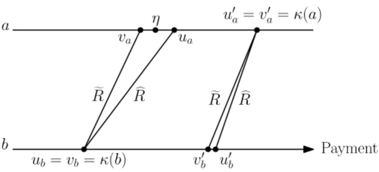
The necessity of the posted-price property and monotonicity has been already ar- gued. The proof of the other direction (ii) ⇒ (i) is rather involved and is provided in Appendix A. We present a sketch of the proof for the case of two alternatives.
Consider the two alternatives case: A = { a b } . Suppose a b (if is empty, the proof is simpler). Fix some > 0 and a domain D that satisfies TP
richness. Let (f p) be a mechanism on this domain that satisfies monotonicity and the posted-price property.
Hence, there are two numbers κ(a) and κ(b) such that for every R ∈ D , we have p(R) = κ(f (R)). Assume, to the contrary, that there is a preference R ∈ D such that f (R) = a and (b κ(b))P(a κ(a)). Then it must be that V
R(a (b κ(b))) < κ(a). Define
η := inf
R:f (R)=a
V
Ra
b κ(b)
By ontoness, there is some R
with f (R
) = b. By monotonicity, we have V
R(a (b κ(b))) ≥ V
R(a (b κ(b))) for every R
with f (R
) = a. Hence, η ≥ V
R(a (b κ(b))) >
κ(b), where the strict inequality follows from the fact that a b and R
respects . Since V
R(a (b κ(b))) < κ(a), we have η < κ(a). We conclude that η is a real number that satisfies
κ(b) < η < κ(a) (1)
We construct two pairs of vectors (u u
) and (v v
) as u
b= v
b= κ(b) u
a= η + δ v
a= η − δ
u
a= v
a= κ(a) u
b= u
b+ κ(a) − u
a+ 3δ v
b= v
b+ κ(a) − v
a+ 1
2 δ
where δ > 0 but sufficiently small. The vectors u, u
, v, and v
are shown in Figure 7 using
an indifference diagram. Using the inequality (1), it is routine to verify that u, u
, v, and
v
respect , (u u
) are
parallel, and (v v
) are
parallel. This uses the fact that for
all values of > 0, we can always find δ > 0 but sufficiently small such that these pairs of
vectors are
parallel. Using TP
richness, we construct two preferences R and R such
that u u
∈ I ( R) and v v
∈ I ( R). By definition of η, there exists a preference R
∗such
that f (R
∗) = a and V
R∗(a (b κ(b))) < η + δ. Since V
R(a (b κ(b))) = η + δ, monotonic-
ity implies that f ( R) = a. Similarly, by the definition of η, we see that f ( R) = b. But by
the definition of u
and v
, we have V
R(b (a κ(a))) = u
b> v
b= V
R(b (a κ(a))), which contradicts monotonicity. A similar argument shows that no manipulation is possible from a preference where b is chosen. The general proof uses similar ideas but it is more involved because A can have more than two alternatives and need not be a complete order.
We make two remarks about Theorem 1 before stating our next result.
R emark 1. Theorem 1 is the analogue of monotonicity-based characterization found in the literature on quasilinear domain. However, there are significant differences as we explain in Section 8. Informally, such a characterization for the quasilinear domain re- quires monotonicity of the allocation rule and a revenue equivalence formula (which is significantly stronger than the posted-price property). Theorem 1 shows that under TP
richness, monotonicity of the mechanism and the posted-price property are equivalent to DSIC. Of course, monotonicity of the mechanism is different from the monotonicity of the allocation rule alone (though they coincide in the quasilinear domain; see Sec- tion 8 for details).
R emark 2. As discussed earlier, TP
richness is a stronger richness requirement than TP
+richness. We give a simple example to show that Theorem 1 may not hold with TP
+richness; of course, if is a complete order, then the two richness notions are equiva- lent.
Example 3. Suppose A = { a b } and is empty. Suppose D = R
+, i.e., the domain is the set of all positive income effect preferences. Fix two numbers κ(a) and κ(b) with κ(a) >
κ(b). Define a subset of PIE preferences as D
∗:= { R ∈ D : V
R(a (b κ(b))) < κ(b) } . Now consider the following mechanism (f p) on D : for every R ∈ D :
f (R) p(R)
=
b κ(b)
if R ∈ D
∗a κ(a)
otherwise.
By definition, (f p) satisfies the posted-price property. To verify monotonicity, pick R such that f (R) = a and R
such that f (R
) = b. The indifference vectors of prefer- ence R are shown in the indifference diagram in Figure 8. Since R
∈ D
∗but R / ∈ D
∗, we get V
R(a (b κ(b))) < κ(b) ≤ V
R(a (b κ(b))). This shows that one of the monotonicity conditions holds: V
R(a (b κ(b))) < V
R(a (b κ(b))). For the other monotonicity con- dition, we use the fact that R, R
satisfy PIE. Using Fact 1, (a) V
R(a (b κ(b))) < κ(b) im- plies V
R(b (a κ(a))) ≥ κ(a) and (b) V
R(a (b κ(b))) ≥ κ(b) implies V
R(b (a κ(a))) ≤ κ(a) (since R satisfies PIE). Combining these two, we get the other monotonicity condi- tion: V
R(b (a κ(b))) ≤ V
R(b (a κ(a))).
However, this mechanism is not DSIC. Since κ(a) > κ(b), there is R / ∈ D
∗such that V
R(b (a κ(a))) = κ(a) > κ(b). As shown in Figure 8, since (f (R) p(R)) = (a κ(a)), we see that R is better off manipulating to a preference in D
∗to get the consumption bundle (b κ(b)).
Note that if is empty, R
+= R (the entire set of preferences). Consider the earlier
mechanism (f p) in Example 3 on D = R . The earlier argument again shows that f is
Figure 8. Indifference diagram of a preference R satisfying PIE with V
R(b (a κ(a))) = κ(a).
Figure 9. Illustration of violation of monotonicity of f when is empty.
not DSIC. We know that Theorem 1 holds in R . Hence, f must violate monotonicity. To see this, consider R and R
as shown in Figure 9. Note that R
violates PIE and f (R) = a, f (R
) = b by definition of f . However, V
R(b (a κ(a))) < V
R(b (a κ(a))). Hence,
monotonicity is violated. ♦
5. A revenue uniqueness theorem
One of the fundamental results in mechanism design with quasilinearity is the revenue equivalence. It helps us to understand why seemingly different auction formats generate the same expected revenue. From a methodological point of view, revenue equivalence allows significant simplification of the optimization problem for maximizing revenue.
D efinition 11. A domain D satisfies revenue equivalence if for every pair of DSIC mechanisms (f p) and (f p) ˆ on D , we have
p(R) − ˆ p(R) = p( R) ˆ − ˆ p( R) ˆ ∀ R R ˆ ∈ D
In other words, if two mechanisms differ from each other only in their payment rules, then the payment rules must be translations of each other. It is well known that Q is a revenue equivalence domain.
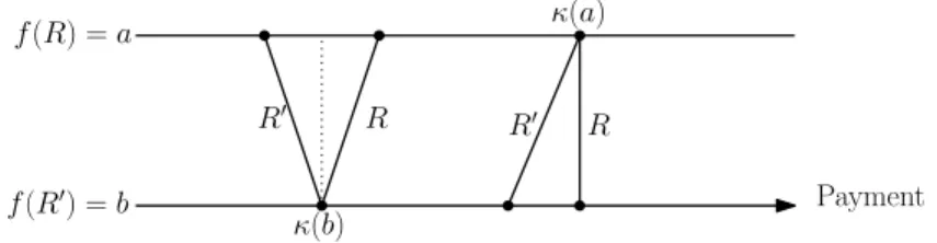
What happens to revenue equivalence without quasilinearity? Consider an exam- ple with four alternatives. Let (f p) and (f p) ˆ be two DSIC mechanisms such that p ˆ is a translation of p. By the posted-price property, we have two maps κ : A → R and
ˆ
κ : A → R corresponding to these two mechanisms. Assume that κ and κ ˆ are transla-
tions of each other. The indifference diagram is shown in Figure 10. As shown in Fig-
ure 10, we can construct two vectors v and v ˆ such that v is to the left of κ and v ˆ is to
Figure 10. Failure of revenue equivalence.
the right of κ. If we can ensure that there exists a preference ˆ R such that v v ˆ ∈ I (R), then we get a contradiction from DSIC as follows: DSIC of (f p) implies that f (R) = a (since (a κ(a))P(x κ(x)) for all x = a) but DSIC of (f p) ˆ implies that f (R) = a (since (x κ(x))P(a ˆ κ(a)) ˆ for all x = a). We show that the existence of such a preference R is guaranteed by TP
+richness even if κ and κ ˆ are not parallel. Hence, we get the following result.
D efinition 12. A domain D satisfies revenue uniqueness if for every pair of DSIC mech- anism (f p) and (f p) ˆ on D , we have p = ˆ p.
T heorem 2. Let > 0. Every domain that satisfies TP
+richness satisfies revenue unique- ness.
P roof . Let D be a domain that satisfies TP
+richness for some > 0. Assume, to the contrary, that there exist two DSIC mechanisms (f p) and (f p
) such that p = p
. DSIC implies that the posted-price property holds; see the discussion immediately af- ter Definition 10. Hence, there exist maps κ and κ
such that κ(f (R)) = p(R) and κ
(f (R)) = p
(R) for all R ∈ D . Since p = p
, we get κ = κ
. We now complete the proof in three steps.
S tep 1. In this step, we show that κ and κ
respect .
8Pick any a b ∈ A and suppose b a. Pick R such that f (R) = a (by ontoness, this is possible). By incentive compatibility, V
R(b (a κ(a))) ≤ κ(b). Since R respects , we have κ(a) < V
R(b (a κ(a))). Combining the two inequalities, we get κ(b) > κ(a) as desired. A similar proof works for κ
.
S tep 2. In this step, we show that either κ > κ
or κ
> κ. Without loss of generality, as- sume that κ(a) > κ
(a) for some a ∈ A. We show that κ(b) > κ
(b) for all b ∈ A. Assume, to the contrary, that κ(b) ≤ κ
(b) for some b ∈ A. Let δ > 0 but sufficiently close to zero.
Define v as v
x:= κ(x) − δ for all x = b and v
b:= κ(b). Since δ is chosen sufficiently small and κ respects (by Step 1), v respects . Further, v
a> κ
(a). By OP richness (which is implied by TP
+richness), there is R ∈ D such that v ∈ I (R).
8
Of course, if is empty, then there is nothing to prove.
For each x = b, we have (b κ(b))P(x κ(x)) by construction of v. Thus, DSIC of (f p) implies f (R) = b. However, since v
a> κ
(a) and κ(b) ≤ κ
(b), we have
a κ
(a) P
b κ(b) R
b κ
(b)
Then DSIC of (f p
) implies f (R) = b. This is a contradiction. Hence, κ(b) > κ
(b) for all b ∈ A.
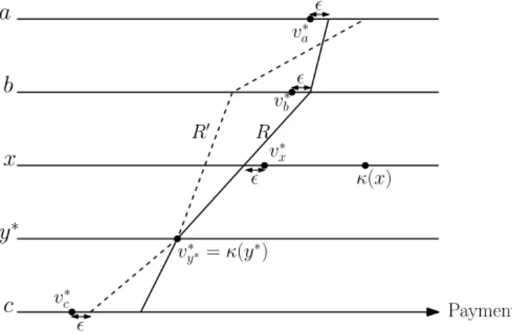
S tep 3. We now complete the proof. Since κ and κ
respect and κ > κ
, Lemma 4 (whose statement and proof are given in Appendix B) implies the existence of vectors v v
∈ R
|A|that respect and are
+parallel. Further, by Lemma 4, there exists a
∗∈ A such that
v
a∗= κ a
∗v
x< κ(x) ∀ x = a
∗and v
a∗= κ
a
∗v
x> κ
(x) ∀ x = a
∗By TP
+richness, there exists a preference R such that v v
∈ I (R). By definition of v
, (x κ
(x))P(a
∗κ
(a
∗)) for all x = a
∗. Since (f p
) is DSIC, we must have f (R) = a
∗. Alter- natively, v
x< κ(x) for all x = a
∗. But v
a∗= κ(a
∗) implies that (a
∗κ(a
∗))P(x κ(x)) for all x = a
∗. Since (f p) is DSIC, we must have f (R) = a
∗. This is a contradiction.
Theorem 2 provides an analogue to a fundamental result in the quasilinear domain.
Once an allocation rule is fixed, in a domain satisfying TP
+richness, DSIC leaves little flexibility in the construction of a payment rule.
6. D oes individual rationality bind ?
A well known result in the screening problem with quasilinearity is that the individual ra- tionality constraint binds for “low types” in the expected revenue-maximizing contract for the principal (Mussa and Rosen 1978). This result leads to a major simplification on obtaining a solution to the optimal contract. In this section, we explore the validity of this result on non-quasilinear domains.
We assume that a
0∈ A is the worst alternative according to and that the IR con- straint is defined with (a
00) being the outside consumption bundle (Definition 3). We state a straightforward lemma on IR below.
L emma 2. Suppose (f p) is a DSIC mechanism. Then it is IR if and only if p(R) ≤ 0 for all R with f (R) = a
0.
P roof . If (f p) is IR, then (a
0p(R))R(a
00) for all R with f (R) = a
0, and this implies that p(R) ≤ 0. For the converse, pick any R with f (R) = a. There exists a R
with f (R
) = a
0. By DSIC, (a p(R))R(a
0p(R
))R(a
00), where the last relation comes from the fact that p(R
) ≤ 0. Hence, (f p) is IR.
Lemma 2 assumes that the range of f includes a
0. If the range of f does not include
a
0, our assumption implies the agent pays zero whenever she exercises her outside op-
tion (a
00). The point of this section is to show that if a
0is in the range of a DSIC and
IR mechanism, we can construct another DSIC and IR mechanism such that IR binds in
the following sense.
D efinition 13. IR binds in a domain D if for every DSIC and IR mechanism (f p) on D , there exists a DSIC and IR mechanism ( f ˆ p) ˆ on D such that
ˆ
p(R) = 0 ∀ R ∈ D such that f (R) ˆ = a
0ˆ
p(R) ≥ p(R) ∀ R ∈ D
If IR binds, we can convert any DSIC and IR mechanism to another DSIC and IR mechanism such that payment for a
0is zero and revenue does not fall.
The IR constraint binds in Q . This can be seen as follows. Pick (f p) that is DSIC and IR. By Lemma 2, we see that p(R) ≤ 0 for all R with f (R) = a
0. By the posted-price property, κ(a
0) = p(R) ≤ 0 for all R with f (R) = a
0. Define p(R) ˆ = p(R) − κ(a
0) for all R.
Since p ˆ is a translation of p and the domain is the quasilinear domain, we see that (f p) ˆ is DSIC and IR. Since κ(a
0) ≤ 0, we have p(R) ˆ ≥ p(R) for all R. Hence, IR binds in Q . A crucial aspect of this simple argument is that we only change p to p ˆ while constructing the new mechanism. The allocation rule f was unchanged. Such an argument does not work if the domain is not Q . Even then, we can establish that IR binds in any domain of preferences.
T heorem 3. IR binds in every domain of preferences.
P roof . Suppose D is a domain of preferences. Let (f p) be a DSIC and IR mechanism defined on D . By the posted-price property, there exists κ : A → R such that κ(f (R)) = p(R) for all R ∈ D . By Lemma 2, we know that κ(a
0) ≤ 0. Let A \ { a
0} = { a
1a
K} and without loss of generality, assume that κ(a
1) ≤ · · · ≤ κ(a
K). We now define another map
˜
κ : A → R as κ(a ˜
0) := 0 and
˜
κ(a
1) := inf
R:f (R)=a1
V
Ra
1a
0κ(a ˜
0) Having defined κ(a ˜
1) κ(a ˜
k), we define
˜
κ(a
k+1) := min
aj∈{a0ak}
inf
R:f (R)=ak+1
V
Ra
k+1a
jκ(a ˜
j)
The mechanism ( f ˜ p) ˜ is defined as follows. For every R, the agent chooses her best consumption bundle according to R from the set { (a
0κ(a ˜
0)) (a
Kκ(a ˜
K)) } , with ties broken in favor of the higher indexed alternative. More formally, for every R, define
M(R) :=
a
jκ(a ˜
j) :
a
jκ(a ˜
j) R
a
kκ(a ˜
k)
∀ a
k∈ A
Then f (R) ˜ := a
if a
∈ M(R) and > j for all a
j∈ M(R) \ { a
} . Further, p(R) ˜ := ˜ κ(a
).
Trivially, ( f ˜ p) ˜ is DSIC. Since κ(a ˜
0) = 0, by Lemma 2, ( f ˜ p) ˜ is IR. We now complete the proof by showing that p(R) ˜ ≥ p(R) for all R.
S tep 1. In this step, we show that κ(a ˜
j) ≥ κ(a
j) for all a
j∈ A. Since (f p) is IR, we know
that κ(a
0) ≤ 0. By definition, 0 = ˜ κ(a
0) ≥ κ(a
0). Now, we prove the step using induction
on the indices: suppose κ(a ˜
j) ≥ κ(a
j) for all a
j∈ { a
0a
k} . Then we observe that
˜
κ(a
k+1) = min
aj∈{a0ak}
inf
R:f (R)=ak+1
V
Ra
k+1a
jκ(a ˜
j)
≥ min
aj∈{a0ak}
inf
R:f (R)=ak+1
V
Ra
k+1a
jκ(a
j)
(by the induction hypothesis)
≥ κ(a
k+1)
where the last inequality follows from the fact that for every R with f (R) = a
k+1, DSIC implies that V
R(a
k+1(a
jκ(a
j)) ≥ κ(a
k+1) for all a
j∈ A.
S tep 2. We now complete the proof. Pick any R ∈ D . Let f (R) = a
k. By definition,
˜
κ(a
k) ≤ V
R(a
k(a
jκ(a ˜
j))) for all j < k. Hence, (a
kκ(a ˜
k))R(a
jκ(a ˜
j)) for all j < k. But then by the tie-breaking rule, f (R) ˜ = a
jfor all j < k. So f (R) ˜ = a
for some ≥ k. Hence, we get
p(R) = κ(a
k) ≤ κ(a ) ≤ ˜ κ(a ) = ˜ p(R)
where the first inequality follows from the fact that ≥ k and the second inequality fol- lows from Step 1.
R emark 3. The allocations rules f and f ˜ in the proof of Theorem 3 can be quite different on an arbitrary domain. They are identical if the domain is Q . However, we can establish a relationship between f and f ˜ . As in the proof of Theorem 3, let A \ { a
0} = { a
1a
K} , and without loss of generality, assume that κ(a
1) ≤ · · · ≤ κ(a
K).
We can show that for any R, f (R) = a
jand f (R) ˜ = a
kimplies k ≥ j. The claim is ob- vious if j = 0. So assume that j > 0. Now pick a
, where < j. By the definition of
˜
κ(a
j), we have κ(a ˜
j) ≤ V
R(a
j(a κ(a ˜ ))). Hence, (a
jκ(a ˜
j))R(a κ(a ˜ )). Further, < j and the tie-breaking rule for f ˜ implies f (R) ˜ = a
. In particular, when is complete with a
Ka
K−1· · · a
1a
0, we have κ(a
1) < · · · < κ(a
K). This implies that f (R) ˜ is assigned an alternative a
ksuch that κ(a
k) > κ(a
j), where f (R) = a
j. Thus, f ˜ assigns
“higher valued” alternatives (i.e., higher in the rank of ) at each preference to increase payments.
9Theorem 3 implies that IR binds in Q and all the other domains discussed in Corol- lary 1. This has implications in solving optimization problems with incentive and indi- vidual rationality constraints as we discuss in the next section.
7. A template for optimal contract design
In this section, we demonstrate the usefulness of the results in the previous section in finding the solution to the optimal contract problem in non-quasilinear environments.
We assume the existence of a
0such that a a
0for all a ∈ A and the IR constraint is defined with (a
00) as the outside option. We fix a domain D . Let μ be a probability
9
We are grateful to an anonymous referee for suggesting this discussion.
measure on D . A mechanism (f
∗p
∗) is optimal if it is a solution to the program (in all the optimization programs below, we assume that a maximum exists)
f:D→Ap:D→R
max
D
p(R) dμ(R) subject to (f p) is DSIC and IR.
Using our results, we show that the optimization program above can be simplified. To do so, we define the notion of a canonical mechanism. For every allocation rule f : D → A, define its canonical payment rule p
f: D → R as
p
f(R) =
⎧ ⎨
⎩
0 if f (R) = a
0R:f (R
inf
)=aV
Ra (a
00)
if f (R) = a = a
0A mechanism (f p) is a canonical mechanism if p = p
f. A canonical mechanism is uniquely defined by the allocation rule only. A canonical mechanism is not necessar- ily DSIC. However, if it is DSIC, then it is IR too, since the payment is zero when a
0is allocated. We show below that an optimal mechanism is a canonical mechanism.
T heorem 4. Suppose D satisfies OP richness. Then an optimal mechanism on D is a canonical mechanism.
Proof. The proof uses the following lemma that characterizes DSIC mechanisms in domains satisfying OP richness.
L emma 3. Suppose D satisfies OP richness and (f p) is a mechanism defined on D . Then (f p) is DSIC if and only if, for every R R
∈ D , we have
p(R) = inf
R:f (R)=f (ˆ R)ˆ
V
Rˆf (R)
f R
p R
Proof. Suppose (f p) satisfies the condition in the statement of the lemma. Then pick any R, R
and we get
p(R) ≤ V
Rf (R)
f R
p R
Hence, (f (R) p(R))R(f (R
) p(R
)), which implies that (f p) is DSIC.
Now suppose (f p) is DSIC. Then DSIC implies, from the necessity of the posted- price property and Step 1 in the proof of Theorem 2, that there exists a map κ : A → R such that κ respects and κ(f (R)) = p(R) for all R. Then pick any a b ∈ A. Choose > 0 but arbitrarily close to zero and consider the following vector v ∈ R
|A|:
v
a= κ(a) + v
x= κ(x) ∀ x = a
Since κ respects and is sufficiently close to zero, v respects . By OP richness, there is a preference R ˆ such that v ∈ I ( R). Since ˆ v
a> κ(a) and v
x= κ(x) for all x = a, DSIC implies that f ( R) ˆ = a. Hence, we have V
Rˆ(a (b κ(b))) = κ(a) + . Taking → 0, we get
κ(a) = inf
R:f (ˆ R)=aˆ
V
Rˆa
b κ(b)
We can now complete the proof of the theorem. By Theorem 3, IR binds. Hence, every optimal mechanism (f p) must have p(R) = 0 if f (R) = a
0. Then, by Lemma 3, OP richness guarantees that for every R with f (R) = a = a
0, we have p(R) = inf
R:f (R)=aV
R(a (a
00)). Hence, p = p
f, and every optimal mechanism is a canonical mechanism.
R emark 4. Theorem 4 assumes that a
0lies in the range of the optimal mechanism. This is without loss of generality for any probability measure that assigns zero probability to a set containing one preference. To see this, suppose (f p) is an optimal mecha- nism such that a
0is not in the range of f . Suppose the range of f is A
:= A \ { a
0}. By the posted-price property, there is a map κ : A
→ R such that for all R with f (R) = a, we have p(R) = κ(f (R)). Then consider the vector v, where v
a0= 0 and v
a= κ(a) for all a ∈ A
. By OP richness, there is a preference R such that v ∈ I (R). By defini- tion, (f (R) p(R))I(a
00). Consider a new mechanism (f
p
) such that f
(R) = a
0and p
(R) = 0, and f
(R
) = f (R
), p
(R
) = p(R
) for all R
= R. Since (f p) is DSIC and IR, the new mechanism (f
p
) is also DSIC. By Lemma 2, the new mechanism (f
p
) sat- isfies IR. Further, the two mechanisms differ at only one preference. By our assumption on the probability measure, the expected revenue from both mechanisms is the same.
10Theorem 4 and Theorem 1 have an immediate corollary that allows us to reduce the search space of our optimal mechanism. First, Theorem 4 shows that we need to search only over canonical mechanisms. Second, Theorem 1 says that if the domain sat- isfies TP
richness for some > 0, we need to search only over canonical mechanisms that satisfy monotonicity. By construction, every DSIC canonical mechanism is IR and, hence, we can get rid of the IR constraint. Further, every canonical mechanism satisfies the posted-price property. Therefore, DSIC can just be replaced by the monotonicity condition of the canonical mechanism. Since a canonical mechanism is uniquely de- fined by the corresponding allocation rule, the search space of the optimal mechanism problem becomes the space of all allocation rules such that the canonical mechanism is monotone. This leads to the following corollary.
Corollary 2. Let > 0. Suppose D satisfies TP
richness. Then every optimal mecha- nism is a solution to the program
max
f:D→A
D
p
f(R) dμ(R) subject to
f p
fis monotone.
This result parallels a similar result in the quasilinear domain. As argued earlier, The- orem 4 holds in the quasilinear domain. We say an allocation rule f is implementable if there exists a payment rule p such that (f p) is DSIC. It is difficult to verify imple- mentability of an allocation rule without quasilinearity (because of the nonseparable nature of allocation and payment in the utility function of the agent). However, if the
10
We are grateful to an anonymous referee for motivating this discussion.
domain is Q , an allocation rule is implementable if and only if it is weakly monotone (Bikhchandani et al. 2006). An allocation rule f (defined on the quasilinear domain) is weakly monotone if for every quasilinear preferences R and R
with f (R) = a and f (R
) = b such that valuation vectors v and v
represent R and R
, respectively, we have v
a− v
b≥ v
a− v
b. As we show later, in the quasilinear domain, a mechanism (f p) is monotone if and only if f is weakly monotone. We also know that if f is implementable on Q , then, by revenue equivalence, we can construct p
fsuch that (f p
f) is DSIC and IR (Heydenreich et al. 2009). Hence, the analogue of the program in Corollary 2 is well known to be the following program on Q :
f:Q→
max
AQ
p
f(R) dμ(R)
subject to f is weakly monotone.
Such a simplification is useful for computing an optimal contract. For instance, in the single object allocation problem, it is standard to solve the unconstrained optimization problem and then verify that the unconstrained optimum satisfies weak monotonicity.
Our program in Corollary 2 has similar features: the search space of the optimal mechanism is only over allocation rules such that the corresponding canonical mech- anism is monotone. Thus, we provide a template for designing optimal mechanisms without quasilinearity. Such a template is useful if the underlying optimization problem is tractable. This depends on the specific domain considered. We now briefly outline how it can be applied to a model with two alternatives.
Suppose A = { a
0a
1} with a
1a
0. In a model, where a single object needs to be al- located, a
0can be thought of as the alternative where the object is not allocated and a
1is the alternative where the object is allocated. To find a revenue-maximizing mecha- nism in such a model, Theorem 4 says that we need to focus on canonical mechanisms that correspond to monotone allocation rules. Given an allocation rule f , the canonical mechanism in this model has a payment rule characterized by
κ
f(a
0) = 0 κ
f(a
1) = inf
R:f (R)=a1