Hilbert Space Embeddings and Metrics on Probability Measures

Hilbert Space Embeddings and Metrics on Probability Measures

Bharath K. Sriperumbudur

Department of Electrical and Computer Engineering University of California, San Diego

La Jolla, CA 92093-0407, USA

Arthur Gretton

MPI for Biological Cybernetics Spemannstraße 38

72076, T¨ubingen, Germany

Kenji Fukumizu

The Institute of Statistical Mathematics 10-3 Midori-cho, Tachikawa

Tokyo 190-8562, Japan

Bernhard Sch¨olkopf

MPI for Biological Cybernetics Spemannstraße 38

72076, T¨ubingen, Germany

Gert R. G. Lanckriet

Department of Electrical and Computer Engineering University of California, San Diego

La Jolla, CA 92093-0407, USA

Editor: Ingo Steinwart

Abstract

A Hilbert space embedding for probability measures has recently been proposed, with applications including dimensionality reduction, homogeneity testing, and independence testing. This embed- ding represents any probability measure as a mean element in a reproducing kernel Hilbert space (RKHS). A pseudometric on the space of probability measures can be defined as the distance be- tween distribution embeddings: we denote this asγk, indexed by the kernel function k that defines the inner product in the RKHS.

We present three theoretical properties ofγk. First, we consider the question of determining the conditions on the kernel k for whichγkis a metric: such k are denoted characteristic kernels. Un- like pseudometrics, a metric is zero only when two distributions coincide, thus ensuring the RKHS embedding maps all distributions uniquely (i.e., the embedding is injective). While previously pub- lished conditions may apply only in restricted circumstances (e.g., on compact domains), and are difficult to check, our conditions are straightforward and intuitive: integrally strictly positive defi- nite kernels are characteristic. Alternatively, if a bounded continuous kernel is translation-invariant onR^d, then it is characteristic if and only if the support of its Fourier transform is the entireR^d. Second, we show that the distance between distributions underγkresults from an interplay between the properties of the kernel and the distributions, by demonstrating that distributions are close in the embedding space when their differences occur at higher frequencies. Third, to understand the

∗. Also at Carnegie Mellon University, Pittsburgh, PA 15213, USA.

nature of the topology induced byγk, we relateγkto other popular metrics on probability measures, and present conditions on the kernel k under whichγkmetrizes the weak topology.

Keywords: probability metrics, homogeneity tests, independence tests, kernel methods, universal kernels, characteristic kernels, Hilbertian metric, weak topology

1. Introduction

The concept of distance between probability measures is a fundamental one and has found many applications in probability theory, information theory and statistics (Rachev, 1991; Rachev and R¨uschendorf, 1998; Liese and Vajda, 2006). In statistics, distances between probability measures are used in a variety of applications, including hypothesis tests (homogeneity tests, independence tests, and goodness-of-fit tests), density estimation, Markov chain monte carlo, etc. As an example, homogeneity testing, also called the two-sample problem, involves choosing whether to accept or reject a null hypothesis H

: P = Q versus the alternative H

: P 6 = Q, using random samples { X

}

and { Y

}

drawn i.i.d. from probability distributions P and Q on a topological space (M,A).

It is easy to see that solving this problem is equivalent to testing H

: γ(P, Q) = 0 versus H

: γ(P,Q) > 0, where γ is a metric (or, more generally, a semi-metric

) on the space of all probability measures defined on M. The problems of testing independence and goodness-of-fit can be posed in an analogous form. In non-parametric density estimation, γ( p

, p

) can be used to study the quality of the density estimate, p

, that is based on the samples { X

}

drawn i.i.d. from p

. Popular examples for γ in these statistical applications include the Kullback-Leibler divergence, the total variation distance, the Hellinger distance (Vajda, 1989)—these three are specific instances of the generalized φ-divergence (Ali and Silvey, 1966; Csisz´ar, 1967)—the Kolmogorov distance (Lehmann and Romano, 2005, Section 14.2), the Wasserstein distance (del Barrio et al., 1999), etc.

In probability theory, the distance between probability measures is used in studying limit theo- rems, the popular example being the central limit theorem. Another application is in metrizing the weak convergence of probability measures on a separable metric space, where the L´evy-Prohorov distance (Dudley, 2002, Chapter 11) and dual-bounded Lipschitz distance (also called the Dudley metric) (Dudley, 2002, Chapter 11) are commonly used.

In the present work, we will consider a particular pseudometric

on probability distributions which is an instance of an integral probability metric (IPM) (M¨uller, 1997). Denoting P the set of all Borel probability measures on (M,A), the IPM between P ∈ P and Q ∈ P is defined as

γ

(P,Q) = sup

f∈F

M

f dP −

M

f dQ

, (1)

where F is a class of real-valued bounded measurable functions on M. In addition to the general application domains discussed earlier for metrics on probabilities, IPMs have been used in proving central limit theorems using Stein’s method (Stein, 1972; Barbour and Chen, 2005), and are popular in empirical process theory (van der Vaart and Wellner, 1996). Since most of the applications listed

1. Given a set M, a metric for M is a function ρ: M×M→R+ such that (i) ∀x,ρ(x,x) =0, (ii)∀x,y,ρ(x,y) = ρ(y,x), (iii)∀x,y,z,ρ(x,z)≤ρ(x,y) +ρ(y,z), and (iv)ρ(x,y) =0⇒x=y. A semi-metric only satisfies (i), (ii) and (iv). A pseudometric only satisfies (i)-(iii) of the properties of a metric. Unlike a metric space(M,ρ), points in a pseudometric space need not be distinguishable: one may haveρ(x,y) =0 for x6=y.

Now, in the two-sample test, though we mentioned thatγis a metric/semi-metric, it is sufficient thatγsatisfies (i) and (iv).

above require γ

to be a metric on P , the choice of F is critical (note that irrespective of F , γ

is a pseudometric on P ). The following are some examples of F for which γ

is a metric.

(a) F = C

(M), the space of bounded continuous functions on (M,ρ), where ρ is a metric (Shorack, 2000, Chapter 19, Definition 1.1).

(b) F =C

(M), the space of bounded ρ-uniformly continuous functions on (M, ρ)—Portmonteau theorem (Shorack, 2000, Chapter 19, Theorem 1.1).

(c) F = { f : k f k

≤ 1 } =: F

, where k f k

= sup

| f (x) | . γ

is called the total variation distance (Shorack, 2000, Chapter 19, Proposition 2.2), which we denote as TV , that is, γ

=: TV .

(d) F = { f : k f k

≤ 1 } =: F

, where k f k

:= sup {| f (x) − f(y) | /ρ(x,y) : x 6 = y in M } . k f k

is the Lipschitz semi-norm of a real-valued function f on M and γ

is called the Kantorovich metric. If (M, ρ) is separable, then γ

equals the Wasserstein distance (Dudley, 2002, Theo- rem 11.8.2), denoted as W := γ

.

(e) F = { f : k f k

≤ 1 } =: F

, where k f k

:= k f k

+ k f k

. γ

is called the Dudley metric (Shorack, 2000, Chapter 19, Definition 2.2), denoted as β := γ

.

(f) F = {1

: t ∈ R

} =: F

. γ

is called the Kolmogorov distance (Shorack, 2000, Theorem 2.4).

(g) F = { e

: ω ∈ R

} =: F

. This choice of F results in the maximal difference between the characteristic functions of P and Q. That γ

is a metric on P follows from the uniqueness theorem for characteristic functions (Dudley, 2002, Theorem 9.5.1).

Recently, Gretton et al. (2007b) and Smola et al. (2007) considered F to be the unit ball in a reproducing kernel Hilbert space (RKHS) H (Aronszajn, 1950), with k as its reproducing kernel (r.k.), that is, F = { f : k f k

≤ 1 } =: F

(also see Chapter 4 of Berlinet and Thomas-Agnan, 2004, and references therein for related work): we denote γ

=: γ

. While we have seen many possible F for which γ

is a metric, F

has a number of important advantages:

• Estimation of γ

: In applications such as hypothesis testing, P and Q are known only through the respective random samples { X

}

and { Y

}

drawn i.i.d. from each, and γ

(P,Q) is estimated based on these samples. One approach is to compute γ

(P, Q) using the empirical measures P

=

∑

δ

and Q

=

∑

δ

, where δ

represents a Dirac measure at x.

It can be shown that choosing F as C

(M), C

(M), F

or F

results in this approach not yielding consistent estimates of γ

(P, Q) for all P and Q (Devroye and Gy¨orfi, 1990). Al- though choosing F = F

or F

yields consistent estimates of γ

(P,Q) for all P and Q when M = R

, the rates of convergence are dependent on d and become slow for large d (Sriperum- budur et al., 2009b). On the other hand, γ

(P

,Q

) is a p

mn/(m + n)-consistent estimator

of γ

(P,Q) if k is measurable and bounded, for all P and Q. If k is translation invariant on

M = R

, the rate is independent of d (Gretton et al., 2007b; Sriperumbudur et al., 2009b), an

important property when dealing with high dimensions. Moreover, γ

is not straightforward

to compute when F is C

(M), C

(M), F

or F

(Weaver, 1999, Section 2.3): by contrast,

γ

(P,Q) is simply a sum of expectations of the kernel k (see (9) and Theorem 1).

• Comparison to φ-divergences: Instead of using γ

in statistical applications, one can also use φ-divergences. However, the estimators of φ-divergences (especially the Kullback-Leibler divergence) exhibit arbitrarily slow rates of convergence depending on the distributions (see Wang et al., 2005; Nguyen et al., 2008, and references therein for details), while, as noted above, γ

(P

, Q

) exhibits good convergence behavior.

• Structured domains: Since γ

is dependent only on the kernel (see Theorem 1) and kernels can be defined on arbitrary domains M (Aronszajn, 1950), choosing F = F

provides the flex- ibility of measuring the distance between probability measures defined on structured domains (Borgwardt et al., 2006) like graphs, strings, etc., unlike F = F

or F

, which can handle only M = R

.

The distance measure γ

has appeared in a wide variety of applications. These include sta- tistical hypothesis testing, of homogeneity (Gretton et al., 2007b), independence (Gretton et al., 2008), and conditional independence (Fukumizu et al., 2008); as well as in machine learning ap- plications including kernel independent component analysis (Bach and Jordan, 2002; Gretton et al., 2005a; Shen et al., 2009) and kernel based dimensionality reduction for supervised learning (Fuku- mizu et al., 2004). In these applications, kernels offer a linear approach to deal with higher order statistics: given the problem of homogeneity testing, for example, differences in higher order mo- ments are encoded as differences in the means of nonlinear features of the variables. To capture all nonlinearities that are relevant to the problem at hand, the embedding RKHS therefore has to be

“sufficiently large” that differences in the embeddings correspond to differences of interest in the distributions. Thus, a natural question is how to guarantee k provides a sufficiently rich RKHS so as to detect any difference in distributions. A second problem is to determine what properties of distributions result in their being proximate or distant in the embedding space. Finally, we would like to compare γ

to the classical integral probability metrics listed earlier, when used to measure convergence of distributions. In the following section, we describe the contributions of the present paper, addressing each of these three questions in turn.

1.1 Contributions

The contributions in this paper are three-fold and explained in detail below.

1.1.1 W

H C

?

Recently, Fukumizu et al. (2008) introduced the concept of a characteristic kernel, that is, a re- producing kernel for which γ

(P,Q) = 0 ⇔ P = Q, P,Q ∈ P , that is, γ

is a metric on P . The corresponding RKHS, H is referred to as a characteristic RKHS. The following are two characteri- zations for characteristic RKHSs that have already been studied in literature:

1. When M is compact, Gretton et al. (2007b) showed that H is characteristic if k is universal in the sense of Steinwart (2001, Definition 4), that is, H is dense in the Banach space of bounded continuous functions with respect to the supremum norm. Examples of such H include those induced by the Gaussian and Laplacian kernels on every compact subset of R

.

2. Fukumizu et al. (2008, 2009a) extended this characterization to non-compact M and showed

that H is characteristic if and only if the direct sum of H and R is dense in the Banach

space of r-integrable (for some r ≥ 1) functions. Using this characterization, they showed

that the RKHSs induced by the Gaussian and Laplacian kernels (supported on the entire R

) are characteristic.

In the present study, we provide alternative conditions for characteristic RKHSs which address several limitations of the foregoing. First, it can be difficult to verify the conditions of denseness in both of the above characterizations. Second, universality is in any case an overly restrictive condition because universal kernels assume M to be compact, that is, they induce a metric only on the space of probability measures that are supported on compact M.

In Section 3.1, we present the simple characterization that integrally strictly positive definite (pd) kernels (see Section 1.2 for the definition) are characteristic, that is, the induced RKHS is characteristic (also see Sriperumbudur et al., 2009a, Theorem 4). This condition is more natural—

strict pd is a natural property of interest for kernels, unlike the denseness condition—and much easier to understand than the characterizations mentioned above. Examples of integrally strictly pd kernels on R

include the Gaussian, Laplacian, inverse multiquadratics, Mat´ern kernel family, B

-splines, etc.

Although the above characterization of integrally strictly pd kernels being characteristic is sim- ple to understand, it is only a sufficient condition and does not provide an answer for kernels that are not integrally strictly pd,

for example, a Dirichlet kernel. Therefore, in Section 3.2, we provide an easily checkable condition, after making some assumptions on the kernel. We present a com- plete characterization of characteristic kernels when the kernel is translation invariant on R

. We show that a bounded continuous translation invariant kernel on R

is characteristic if and only if the support of the Fourier transform of the kernel is the entire R

. This condition is easy to check compared to the characterizations described above. An earlier version of this result was provided by Sriperumbudur et al. (2008): by comparison, we now present a simpler and more elegant proof.

We also show that all compactly supported translation invariant kernels on R

are characteristic.

Note, however, that the characterization of integral strict positive definiteness in Section 3.1 does not assume M to be R

nor k to be translation invariant.

We extend the result of Section 3.2 to M being a d-Torus, that is, T

= S

× . . .

× S

≡ [0,2π)

, where S

is a circle. In Section 3.3, we show that a translation invariant kernel on T

is characteristic if and only if the Fourier series coefficients of the kernel are positive, that is, the support of the Fourier spectrum is the entire Z

. The proof of this result is similar in flavor to the one in Section 3.2.

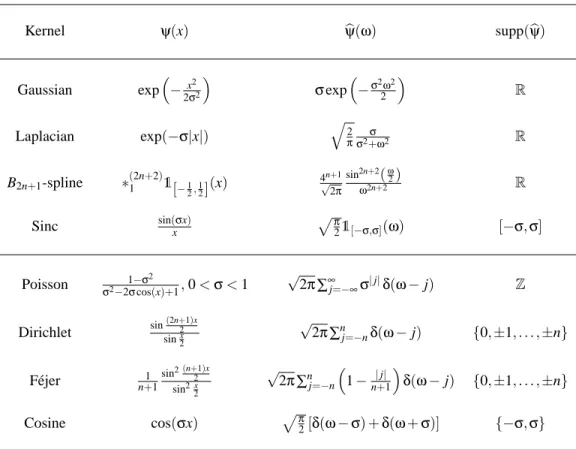
As examples, the Poisson kernel can be shown to be characteristic, while the Dirichlet kernel is not.

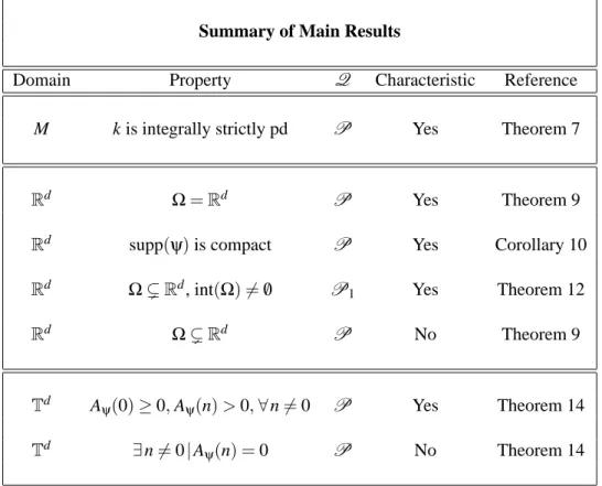
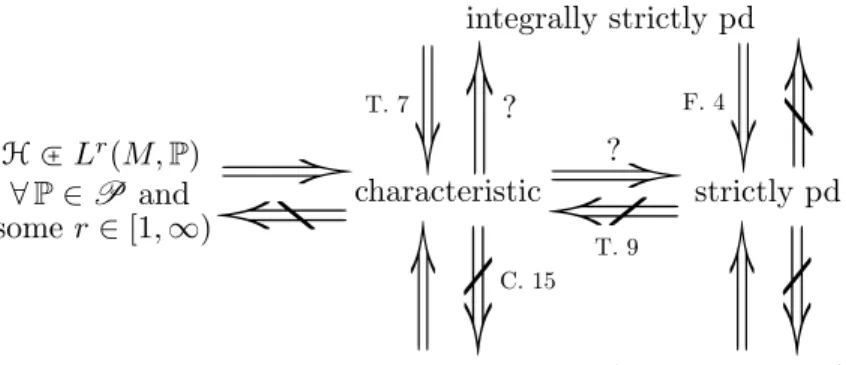
Based on the discussion so far, it is clear that the characteristic property of k can be determined in many ways. In Section 3.4, we summarize the relations between various kernel families (e.g., the universal kernels and the strictly pd kernels), and show how they relate in turn to characteristic kernels. A summary is depicted in Figure 1.

1.1.2 D

D

S

γ

As we have seen, the characteristic property of a kernel is critical in distinguishing between distinct probability measures. Suppose, however, that for a given characteristic kernel k and for any ε > 0, there exist P and Q, P 6 = Q, such that γ

(P, Q) < ε. Though k distinguishes between such P and Q, it can be difficult to tell the distributions apart in applications (even with characteristic kernels), since P and Q are then replaced with finite samples, and the distance between them may not be

2. It can be shown that integrally strictly pd kernels are strictly pd (see Footnote 4). Therefore, examples of kernels that are not integrally strictly pd include those kernels that are not strictly pd.

statistically significant (Gretton et al., 2007b). Therefore, given a characteristic kernel, it is of interest to determine the properties of distributions P and Q that will cause their embeddings to be close. To this end, in Section 4, we show that given a kernel k (see Theorem 19 for conditions on the kernel), for any ε > 0, there exists P 6 = Q (with non-trivial differences between them) such that γ

(P, Q) < ε. These distributions are constructed so as to differ at a sufficiently high frequency, which is then penalized by the RKHS norm when computing γ

.

1.1.3 W

D

γ

M

W

T

P ?

Given γ

, which is a metric on P , a natural question of theoretical and practical importance is

“how is γ

related to other probability metrics, such as the Dudley metric (β), Wasserstein distance (W ), total variation metric (TV ), etc?” For example, in applications like density estimation, where the unknown density is estimated based on finite samples drawn i.i.d. from it, the quality of the estimate is measured by computing the distance between the true density and the estimated density.

In such a setting, given two probability metrics, ρ

and ρ

, one might want to use the stronger

of the two to determine this distance, as the convergence of the estimated density to the true density in the stronger metric implies the convergence in the weaker metric, while the converse is not true.

On the other hand, one might need to use a metric of weaker topology (i.e., coarser topology) to show convergence of some estimators, as the convergence might not occur w.r.t. a metric of strong topology. Clarifying and comparing the topology of a metric on the probabilities is, thus, important in the analysis of density estimation. Based on this motivation, in Section 5, we analyze the relation between γ

and other probability metrics, and show that γ

is weaker than all these other metrics.

It is well known in probability theory that β is weaker than W and TV , and it metrizes the weak topology (we will provide formal definitions in Section 5) on P (Shorack, 2000; Gibbs and Su, 2002). Since γ

is weaker than all these other probability metrics, that is, the topology induced by γ

is coarser than the one induced by these metrics, the next interesting question to answer would be, “When does γ

metrize the weak topology on P ?” In other words, for what k, does the topology induced by γ

coincide with the weak topology? Answering this question would show that γ

is equivalent to β, while it is weaker than W and TV . In probability theory, the metrization of weak topology is of prime importance in proving results related to the weak convergence of probability measures. Therefore, knowing the answer to the above question will help in using γ

as a theoretical tool in probability theory. To this end, in Section 5, we show that universal kernels on compact (M,ρ) metrize the weak topology on P . For the non-compact setting, we assume M = R

and provide sufficient conditions on the kernel such that γ

metrizes the weak topology on P .

In the following section, we introduce the notation and some definitions that are used throughout the paper. Supplementary results used in proofs are collected in Appendix A.

1.2 Definitions and Notation

For a measurable space, M and µ a Borel measure on M, L

(M, µ) denotes the Banach space of r-power (r ≥ 1) µ-integrable functions. We will also use L

(M) for L

(M,µ) and dx for dµ(x) if µ is

3. Two metricsρ1: Y×Y→R+andρ2: Y×Y→R+are said to be equivalent ifρ1(x,y) =0⇔ρ2(x,y) =0,∀x,y∈Y . On the other hand,ρ1is said to be stronger thanρ2ifρ1(x,y) =0⇒ρ2(x,y) =0,∀x,y∈Y but not vice-versa. If ρ1is stronger thanρ2, then we sayρ2is weaker thanρ1. Note that ifρ1is stronger (resp. weaker) thanρ2, then the topology induced byρ1is finer (resp. coarser) than the one induced byρ2.

the Lebesgue measure on M ⊂ R

. C

(M) denotes the space of all bounded, continuous functions on M. The space of all r-continuously differentiable functions on M is denoted by C

(M), 0 ≤ r ≤ ∞.

For x ∈ C, x represents the complex conjugate of x. We denote as i the imaginary unit √

− 1.

For a measurable function f and a signed measure P, P f :=

f dP =

f (x) d P(x). δ

repre- sents the Dirac measure at x. The symbol δ is overloaded to represent the Dirac measure, the Dirac- delta distribution, and the Kronecker-delta, which should be distinguishable from the context. For M = R

, the characteristic function, φ

of P ∈ P is defined as φ

(ω) :=

e

dP(x), ω ∈ R

.

Support of a Borel measure: The support of a finite regular Borel measure, µ on a Hausdorff space, M is defined to be the closed set,

supp(µ) := M \

{ U ⊂ M : U is open, µ(U) = 0 } . (2) Vanishing at infinity and C

(M): A complex function f on a locally compact Hausdorff space M is said to vanish at infinity if for every ε > 0 there exists a compact set K ⊂ M such that | f (x) | < ε for all x ∈ / K. The class of all continuous f on M which vanish at infinity is denoted as C

(M).

Holomorphic and entire functions: Let D ⊂ C

be an open subset and f : D → C be a function.

f is said to be holomorphic (or analytic) at the point z

∈ D if f

(z

) := lim

z→z0

f (z

) − f (z) z

− z

exists. Moreover, f is called holomorphic if it is holomorphic at every z

∈ D. f is called an entire function if f is holomorphic and D = C

.

Positive definite and strictly positive definite: A function k : M × M → R is called positive definite (pd) if, for all n ∈ N, α

, . . . , α

∈ R and all x

, . . . , x

∈ M, we have

∑

α

α

k(x

, x

) ≥ 0. (3) Furthermore, k is said to be strictly pd if, for mutually distinct x

, . . . , x

∈ X , equality in (3) only holds for α

= ··· = α

= 0. ψ is said to be a positive definite function on R

if k(x,y) = ψ(x − y) is positive definite.

Integrally strictly positive definite: Let M be a topological space. A measurable and bounded kernel, k is said to be integrally strictly positive definite if

Z Z

M

k(x,y) dµ(x) dµ(y) > 0, for all finite non-zero signed Borel measures µ defined on M.

The above definition is a generalization of integrally strictly positive definite functions on R

(Stewart, 1976, Section 6):

k(x,y) f (x) f (y) dx dy > 0 for all f ∈ L

(R

), which is the strictly positive definiteness of the integral operator given by the kernel. Note that the above definition is not equivalent to the definition of strictly pd kernels: if k is integrally strictly pd, then it is strictly pd, while the converse is not true.

4. Suppose k is not strictly pd. This means for some n∈Nand for mutually distinct x1, . . . ,xn∈M, there exists R∋αj6=0 for some j∈ {1, . . . ,n}such that∑ⁿj,l=1αjαlk(xj,x_l) =0. By defining µ=∑ⁿj=1αjδx_j, it is easy to see that there exists µ6=0 such that^RR_Mk(x,y)dµ(x)dµ(y) =0, which means k is not integrally strictly pd. Therefore, if k is integrally strictly pd, then it is strictly pd. However, the converse is not true. See Steinwart and Christmann (2008, Proposition 4.60, Theorem 4.62) for an example.

Fourier transform in R

: For f ∈ L

(R

), b f and f

represent the Fourier transform and inverse Fourier transform of f respectively, defined as

b f (y) := 1 (2π)

Z

R^d

e

f (x) dx, y ∈ R

, (4) f

(x) := 1

(2π)

R^d

e

f (y) dy, x ∈ R

. (5) Convolution: If f and g are complex functions in R

, their convolution f ∗ g is defined by

( f ∗ g)(x) :=

Z

R^d

f (y)g(x − y) dy,

provided that the integral exists for almost all x ∈ R

, in the Lebesgue sense. Let µ be a finite Borel measure on R

and f be a bounded measurable function on R

. The convolution of f and µ, f ∗ µ, which is a bounded measurable function, is defined by

( f ∗ µ)(x) :=

Z

R^d

f (x − y) dµ(y).

Rapidly decaying functions, D

and S

: Let D

be the space of compactly supported infinitely differentiable functions on R

, that is, D

= { f ∈ C

(R

) | supp( f ) is bounded } , where supp( f ) = cl { x ∈ R

| f (x) 6 = 0 }

. A function f : R

→ C is said to decay rapidly, or be rapidly decreasing, if for all N ∈ N,

sup

kαk¹≤N

sup

x∈R^d

(1 + k x k

)

| (T

f )(x) | < ∞,

where α = (α

, . . . ,α

) is an ordered d-tuple of non-negative α

, k α k

= ∑

α

and T

=

1 i ∂

∂x1

···

1 i ∂

∂xd

. S

, called the Schwartz class, denotes the vector space of rapidly decreasing functions. Note that D

⊂ S

. Also, for any p ∈ [1,∞], S

⊂ L

(R

). It can be shown that for any f ∈ S

, b f ∈ S

and f

∈ S

(see Folland, 1999, Chapter 9 and Rudin, 1991, Chapter 6 for details).

Distributions, D

d

: A linear functional on D

which is continuous with respect to the Fr´echet topology (see Rudin, 1991, Definition 6.3) is called a distribution in R

. The space of all distribu- tions in R

is denoted by D

d

.

As examples, if f is locally integrable on R

(this means that f is Lebesgue measurable and

K

| f (x) | dx < ∞ for every compact K ⊂ R

), then the functional D

defined by D

(ϕ) =

R^d

f (x)ϕ(x) dx, ϕ ∈ D

, (6)

is a distribution. Similarly, if µ is a Borel measure on R

, then D

(ϕ) =

R^d

ϕ(x) dµ(x), ϕ ∈ D

, defines a distribution D

in R

, which is identified with µ.

Support of a distribution: For an open set U ⊂ R

, D

(U) denotes the subspace of D

consisting of the functions with support contained in U . Suppose D ∈ D

d

. If U is an open set of R

and if

D(ϕ) = 0 for every ϕ ∈ D

(U ), then D is said to vanish or be null in U . Let W be the union of all open U ⊂ R

in which D vanishes. The complement of W is the support of D.

Tempered distributions, S

d

and Fourier transform on S

d

: A linear continuous functional (with respect to the Fr´echet topology) over the space S

is called a tempered distribution and the space of all tempered distributions in R

is denoted by S

d

. For example, every compactly supported distribution is tempered.

For any f ∈ S

d

, the Fourier and inverse Fourier transforms are defined as b f (ϕ) := f ( ϕ), ˆ ϕ ∈ S

,

f

(ϕ) := f (ϕ

), ϕ ∈ S

,

respectively. The Fourier transform is a linear, one-to-one, bicontinuous mapping from S

to S

d

. For complete details on distribution theory and Fourier transforms of distributions, we refer the reader to Folland (1999, Chapter 9) and Rudin (1991, Chapter 6).

2. Hilbert Space Embedding of Probability Measures

Embeddings of probability distributions into reproducing kernel Hilbert spaces were introduced in the late 70’s and early 80’s, generalizing the notion of mappings of individual points: see Berlinet and Thomas-Agnan (2004, Chapter 4) for a survey. Following Gretton et al. (2007b) and Smola et al.

(2007), γ

can be alternatively expressed as a pseudometric between such distribution embeddings.

The following theorem describes this relation.

Theorem 1 Let P

:= { P ∈ P :

p

k(x, x) dP(x) < ∞ } , where k is measurable on M. Then for any P,Q ∈ P

,

γ

(P,Q) =

M

k( · ,x) dP(x) −

M

k( · ,x) dQ(x)

=: k Pk − Qk k

, (7) where H is the RKHS generated by k.

Proof Let T

: H → R be the linear functional defined as T

[ f ] :=

f (x) dP(x) with k T

k :=

sup

kfk^H

. Consider

| T

[ f ] | =

M

f dP ≤

Z

M

| f(x) | dP(x) =

M

|h f, k( · , x) i

| dP(x) ≤

M

p k(x, x) k f k

dP(x),

which implies k T

k < ∞, ∀ P ∈ P

, that is, T

is a bounded linear functional on H . Therefore, by the Riesz representation theorem (Reed and Simon, 1980, Theorem II.4), for each P ∈ P

, there exists a unique λ

∈ H such that T

[ f ] = h f ,λ

i

, ∀ f ∈ H. Let f = k( · ,u) for some u ∈ M. Then, T

[k( · ,u)] = h k( · ,u),λ

i

= λ

(u), which implies λ

=

k( · , x) dP(x) =: Pk. Therefore, with

| P f − Q f | = | T

[ f ] − T

[ f ] | = |h f ,λ

i

− h f ,λ

i

| = |h f ,λ

− λ

i

| , we have

γ

(P, Q) = sup

kfk^H≤1

| P f − Q f | = k λ

− λ

k

= k Pk − Qk k

.

Note that this holds for any P, Q ∈ P

.

Given a kernel, k, (7) holds for all P ∈ P

. However, in practice, especially in statistical inference applications, it is not possible to check whether P ∈ P

as P is not known. Therefore, one would prefer to have a kernel such that

Z

M

p k(x, x) dP(x) < ∞, ∀ P ∈ P . (8)

The following proposition shows that (8) is equivalent to the kernel being bounded. Therefore, combining Theorem 1 and Proposition 2 shows that if k is measurable and bounded, then γ

(P,Q) = k Pk − Qk k

for any P,Q ∈ P .

Proposition 2 Let f be a measurable function on M. Then

f (x) dP(x) < ∞ for all P ∈ P if and only if f is bounded.

Proof One direction is straightforward because if f is bounded, then

f(x) dP(x) < ∞ for all P ∈ P . Let us consider the other direction. Suppose f is not bounded. Then there exists a sequence { x

} ⊂ M such that f (x

)

−→

∞. By taking a subsequence, if necessary, we can assume f (x

) > n

for all n. Then, A := ∑

f(xn)

< ∞. Define a probability measure P on M by P = ∑

δ

, where δ

is a Dirac measure at x

. Then,

f (x) dP(x) =

∑

f(xn)

= ∞, which means if f is not bounded, then there exists a P ∈ P such that

f(x) dP(x) = ∞.

The representation of γ

in (7) yields the embedding, Π : P → H P 7→

Z

M

k( · ,x) dP(x),

as proposed by Berlinet and Thomas-Agnan (2004, Chapter 4, Section 1.1) and Gretton et al.

(2007b); Smola et al. (2007). Berlinet and Thomas-Agnan derived this embedding as a general- ization of δ

7→ k( · , x), while Gretton et al. arrived at the embedding by choosing F = F

in (1).

Since γ

(P, Q) = k Π[P] − Π[Q] k

, the question “When is γ

a metric on P ?” is equivalent to the question “When is Π injective?” Addressing these questions is the central focus of the paper and is discussed in Section 3.

Before proceeding further, we present a number of equivalent representations of γ

, which will improve our understanding of γ

and be helpful in its computation. First, Gretton et al. have shown the reproducing property of k leads to

γ

(P, Q) =

M

k( · ,x) dP(x) −

M

k( · ,x) dQ(x)

2

H

=

M

k( · ,x) dP(x) −

M

k( · ,x) dQ(x),

M

k( · ,y) dP(y) −

M

k( · , y) dQ(y)

H

=

M

k( · ,x) dP(x),

M

k( · ,y) dP(y)

H

+

M

k( · ,x) dQ(x),

M

k( · , y) dQ(y)

H

− 2

M

k( · ,x) dP(x),

M

k( · ,y) dQ(y)

H (a)

=

Z Z

M

k(x,y) dP(x) dP(y) +

M

k(x,y) dQ(x) dQ(y)

− 2

M

k(x,y) dP(x) dQ(y) (9)

=

M

k(x,y) d(P − Q)(x) d(P − Q)(y), (10)

where (a) follows from the fact that

f (x) dP(x) = h f ,

k( · ,x) dP(x) i

for all f ∈ H , P ∈ P (see proof of Theorem 1), applied with f =

k( · ,y) dP(y). As motivated in Section 1, γ

is a straightforward sum of expectations of k, and can be computed easily, for example, using (9) either in closed form or using numerical integration techniques, depending on the choice of k, P and Q. It is easy to show that, if k is a Gaussian kernel with P and Q being normal distributions on R

, then γ

can be computed in a closed form (see Song et al., 2008 and Sriperumbudur et. al., 2009b, Section III-C for examples). In the following corollary to Theorem 1, we prove three results which provide a nice interpretation for γ

when M = R

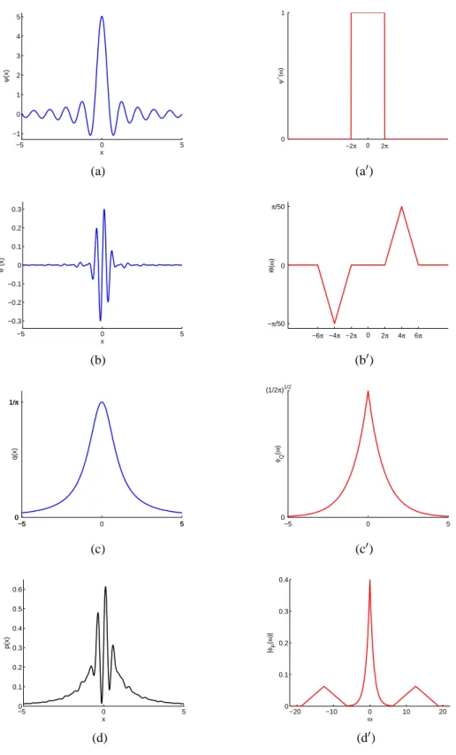
and k is translation invariant, that is, k(x,y) = ψ(x − y), where ψ is a positive definite function. We provide a detailed explanation for Corollary 4 in Remark 5.

Before stating the results, we need a famous result due to Bochner, that characterizes ψ. We quote this result from Wendland (2005, Theorem 6.6).

Theorem 3 (Bochner) A continuous function ψ : R

→ R is positive definite if and only if it is the Fourier transform of a finite nonnegative Borel measure Λ on R

, that is,

ψ(x) =

R^d

e

dΛ(ω), x ∈ R

. (11)

Corollary 4 (Different interpretations of γ

) (i) Let M = R

and k(x,y) = ψ(x − y), where ψ : M → R is a bounded, continuous positive definite function. Then for any P, Q ∈ P ,

γ

(P, Q) = r

R^d

| φ

(ω) − φ

(ω) |

dΛ(ω) =: k φ

− φ

k

, (12) where φ

and φ

represent the characteristic functions of P and Q respectively.

(ii) Suppose θ ∈ L

(R

) is a continuous bounded positive definite function and

θ(x) dx = 1. Let ψ(x) := ψ

(x) = t

θ(t

x), t > 0. Assume that p and q are bounded uniformly continuous Radon- Nikodym derivatives of P and Q w.r.t. the Lebesgue measure, that is, dP = p dx and dQ = q dx.

Then,

lim

γ

(P,Q) = k p − q k

. (13) In particular, if | θ(x) | ≤ C(1 + k x k

)

for some C, ε > 0, then (13) holds for all bounded p and q (not necessarily uniformly continuous).

(iii) Suppose ψ ∈ L

(R

) and p

ψ b ∈ L

(R

). Then,

γ

(P,Q) = (2π)

k Φ ∗ P − Φ ∗ Q k

, (14) where Φ := p

ψ b

and dΛ = (2π)

ψ b dω. Here, Φ ∗ P represents the convolution of Φ and P.

Proof (i) Let us consider (10) with k(x, y) = ψ(x − y). Then, we have γ

(P, Q) =

Z Z

R^d

ψ(x − y) d(P − Q)(x) d(P − Q)(y)

(a)

=

R^d

e

dΛ(ω) d(P − Q)(x) d(P − Q)(y)

(b)

=

R^d

e

d(P − Q)(x)

R^d

e

d(P − Q)(y) dΛ(ω)

=

R^d

(φ

(ω) − φ

(ω))

φ

(ω) − φ

(ω)

dΛ(ω) =

R^d

| φ

(ω) − φ

(ω) |

dΛ(ω),

where Bochner’s theorem (Theorem 3) is invoked in (a), while Fubini’s theorem (Folland, 1999, Theorem 2.37) is invoked in (b).

(ii) Consider (9) with k(x,y) = ψ

(x − y), γ

(P,Q) =

Z Z

R^d

ψ

(x − y)p(x) p(y) dx dy +

R^d

ψ

(x − y)q(x)q(y) dx dy

− 2

R^d

ψ

(x − y)p(x)q(y) dx dy

=

R^d

(ψ

∗ p)(x)p(x) dx +

R^d

(ψ

∗ q)(x)q(x) dx − 2

R^d

(ψ

∗ q)(x) p(x) dx. (15) Note that lim

R

R^d

(ψ

∗ p)(x) p(x) dx =

lim

(ψ

∗ p)(x)p(x) dx, by invoking the dominated convergence theorem. Since p is bounded and uniformly continuous, by Theorem 25 (see Ap- pendix A), we have p ∗ ψ

→ p uniformly as t → 0, which means lim

(ψ

∗ p)(x) p(x) dx =

R^d

p

(x) dx. Using this in (15), we have

t

lim

γ

(P, Q) =

R^d

( p

(x) + q

(x) − 2p(x)q(x)) dx = k p − q k

.

Suppose | θ(x) | ≤ (1 + k x k

)

for some C, ε > 0. Since p ∈ L

(R

), by Theorem 26 (see Ap- pendix A), we have ( p ∗ ψ

)(x) → p(x) as t → 0 for almost every x. Therefore lim

R

R^d

(ψ

∗ p)(x) p(x) dx =

p

(x) dx and the result follows.

(iii) Since ψ is positive definite, ψ b is nonnegative and therefore p

ψ b is valid. Since p

ψ b ∈ L

(R

), Φ exists. Define φ

:= φ

− φ

. Now, consider

k Φ ∗ P − Φ ∗ Q k

=

R^d

| (Φ ∗ (P − Q))(x) |

dx

=

R^d

R^d

Φ(x − y) d(P − Q)(y)

2

dx

= 1

(2π)

R^d

Z Z

R^d

q

ψ(ω) b e

dω d(P − Q)(y)

2

dx

(c)

= 1 (2π)

Z

R^d

R^d

q

ψ(ω)(φ b

(ω) − φ

(ω))e

dω

2

dx

= 1

(2π)

R^d

q

ψ(ω) b q

ψ(ξ) b φ

(ω) φ

(ξ) e

dω dξdx

(d)

=

R^d

q

ψ(ω) b q

ψ(ξ) b φ

(ω) φ

(ξ) 1

(2π)

R^d

e

dx

dω dξ

=

R^d

q

ψ(ω) b q

ψ(ξ) b φ

(ω) φ

(ξ) δ(ω − ξ) dω dξ

=

R^d

ψ(ω) b | φ

(ω) − φ

(ω) |

dω

= (2π)

γ

(P, Q),

where (c) and (d) are obtained by invoking Fubini’s theorem.

Remark 5 (a) (12) shows that γ

is the L

-distance between the characteristic functions of P and Q computed w.r.t. the non-negative finite Borel measure, Λ, which is the Fourier transform of ψ. If ψ ∈ L

(R

), then (12) rephrases the well known fact (Wendland, 2005, Theorem 10.12) that for any

f ∈ H ,

k f k

=

R^d

| b f (ω) |

ψ(ω) b dω. (16)

Choosing f = (P − Q) ∗ ψ in (16) yields b f = (φ

− φ

) ψ b and therefore the result in (12).

(b) Suppose dΛ(ω) = (2π)

dω. Assume P and Q have p and q as Radon-Nikodym derivatives w.r.t. the Lebesgue measure, that is, dP = p dx and dQ = q dx. Using these in (12), it can be shown that γ

(P,Q) = k p − q k

. However, this result should be interpreted in a limiting sense as mentioned in Corollary 4(ii) because the choice of dΛ(ω) = (2π)

dω implies ψ(x) = δ(x), which does not satisfy the conditions of Corollary 4(i). It can be shown that ψ(x) = δ(x) is obtained in a limiting sense (Folland, 1999, Proposition 9.1): ψ

→ δ in D

d

as t → 0.

(c) Choosing θ(x) = (2π)

e

in Corollary 4(ii) corresponds to ψ

being a Gaussian kernel (with appropriate normalization such that

ψ

(x) dx = 1). Therefore, (13) shows that as the bandwidth, t of the Gaussian kernel approaches zero, γ

approaches the L

-distance between the densities p and q. The same result also holds for choosing ψ

as the Laplacian kernel, B

-spline, inverse multiquadratic, etc. Therefore, γ

(P,Q) can be seen as a generalization of the L

-distance between probability measures, P and Q.

(d) The result in (13) holds if p and q are bounded and uniformly continuous. Since any condition on P and Q is usually difficult to check in statistical applications, it is better to impose conditions on ψ rather than on P and Q. In Corollary 4(ii), by imposing additional conditions on ψ

, the result in (13) is shown to hold for all P and Q with bounded densities p and q. The condition,

| θ(x) | ≤ C(1 + k x k

)

for some C, ε > 0, is, for example, satisfied by the inverse multiquadratic kernel, θ(x) = C(1 e + k x k

)

, x ∈ R

, τ > d/2, where C e =

(1 + k x k

)

dx

.

(e) The result in Corollary 4(ii) has connections to the kernel density estimation in L

-sense using Parzen windows (Rosenblatt, 1975), where ψ can be chosen as the Parzen window: see Gretton et al.

(2007a, Section 7.1) for further discussion. Note in particular that when γ

is used in a homogeneity test, a constant kernel bandwidth results in a faster decrease of the Type II error with increasing sample size (Anderson et al., 1994, p. 43). A decreasing bandwidth is required for a consistent estimate of k p − q k

, however.

(f) (14) shows that γ

is proportional to the L

-distance between Φ ∗ P and Φ ∗ Q. Let Φ be such that Φ is nonnegative and Φ ∈ L

(R

). Then, defining Φ e := (

Φ(x) dx)

Φ = Φ/ p

ψ(0) = b (

ψ(x) dx)

Φ and using this in (14), we have

γ

(P,Q) = (2π)

q ψ(0) b

e Φ ∗ P − Φ e ∗ Q

. (17)

The r.h.s. of (17) can be interpreted as follows. Let X , Y and N be independent random variables

such that X ∼ P, Y ∼ Q and N ∼ Φ. This means e γ

is proportional to the L

-distance computed

between the densities associated with the perturbed random variables, X + N and Y + N. Note

that k p − q k

is the L

-distance between the densities of X and Y . Examples of ψ that satisfy

the conditions in Corollary 4(iii) in addition to the conditions on Φ as mentioned here include the