1. Introduction
The vertical distribution of phytoplankton community in the water column is highly hetero-geneous in response to the small-scale physical hydrodynamic changes such as water mass sta-bility(MELLARD et al., 2011), vertical mixing (MAZNAHet al., 2016),and the availability of light (TILZER and GOLDMAN, 1978). Variations of the abiotic water conditions occur naturally at differ-ent timescales throughout the day(GAST et al., 2014),related with the periodic oscillations of the tidal currents(BLAUWet al., 2012),which in turn influence the short-term changes in the phyto-plankton community.
High-resolution observations on fine-scale spatial and temporal
heterogeneity of phytoplankton communities using FlowCAM
KHINKHINGYI1), Takuo OMURA2, 3)*, Rie NAKAMURA3)and Yuji TANAKA1, 2)
Abstract: To understand the fine-scale spatio-temporal phytoplankton dynamics with reference
to the environmental properties of the water column, high-frequency samplings every 4 h, at 0. 5Ȃ2 m depth intervals using a submersible pump was conducted in Tateyama Bay, Japan, for 24 h from 12 h of 12 May to 08 h of 13 May 2017. The FlowCAM, which is an automatic device, was used to identify, count and size the phytoplankton. As a result, the phytoplankton distribution significantly varied within a few meters and a short timescale(several hours)of a day. For ex-ample, Thalassiosira sp. and Prorocentrum minimum were detected at all sampling depths and times rather evenly, but the water-column total abundance of Dactyliosolen fragilissimus and Scrippsiella trochoidea significantly decreased after the 2nd set of the samplings. Species-specific vertical distributions were various but related to the condition(strength and depth)of the thermocline at each sampling time. These phytoplankton species-specific distributions and variations in the composition reflect the eco-physiological characteristics and size structure of phytoplankton and the short-term hydrodynamic events. The high value of chlorophyll-a in the bottom layers was not only from the phytoplankton but also from the fluorescence of the aggre-gate particles.
Keywords : phytoplankton, spatio-temporal distribution, FlowCAM, fine-scale sampling
1)Graduate School of Marine Science and Technolo-gy, Tokyo University of Marine Science and Technology, 4Ȃ5Ȃ7 Konan, Minato, Tokyo 108Ȃ 8477, Japan
2)Department of Ocean Sciences, School of Marine Resources and Environment, Tokyo University of Marine Science and Technology, 4Ȃ5Ȃ7 Konan, Minato, Tokyo 108Ȃ8477, Japan
3)Laboratory of Aquatic Science Consultant, 2Ȃ30Ȃ 17 Higashikamata, Ota, Tokyo 144Ȃ0031, Japan *Corresponding author:Takuo OMURA
Tel: 03Ȃ6428Ȃ6715 Fax: 03Ȃ6428Ȃ6716 E-mail: [email protected]
1)Institute of Marine Science, Burapha University, Bangsaen, Chon Buri 20131, Thailand
2)Department of Aquatic Science, Faculty of Sci-ence, Burapha University, Bangsaen, Chon Buri 20131, Thailand
3)Atmosphere and Ocean Research Institute, The
University of Tokyo, 5Ȃ1Ȃ5, Kashiwanoha, Kashi-wa, Chiba 277Ȃ8564, Japan
*Corresponding author: Thidarat Noiraksar Tel: + 66(0)38 391671
Fax: + 66(0)38 391674
Despite the relationship between environmen-tal properties, ecological characteristics and fine-scale phytoplankton dynamics has been reported by previous studies(e.g. DEKSHENIEKSet al., 2001; GERVAISet al., 2003; LUNVENet al., 2005; CARON et al., 2008),it is still remaining to explore how do phytoplankton fluctuate throughout the entire water column, in a short timescale of the day. Hence, we here conducted a series of pump sam-plings throughout the whole vertical water col-umn, at a relatively fine-scale of 0.5Ȃ2 m depth in-terval, every 4 h, dealing with the physical characteristics of the water column. The aim was to understand the precise spatial and tempo-ral distributions of phytoplankton abundance, composition and the size structure, together with the particle distribution data, and thus pro-vide relevant information about the short-term changes in the phytoplankton vertical distribu-tion and the community dynamics. In the case of monitoring the high-resolution field survey data, traditional microscopic examination is time-consuming. To overcome this difficulty, we
de-ployed an automatic device FlowCAM(the Flow Cytometer And Microscope), which has com-bined capabilities of flow cytometry, microscopy and image analysis(SIERACKI et al., 1998). This apparatus counts and photographs particles moving in a fluid flow. To create this flow, the water sample is drawn into the instrument by means of a peristaltic pump. A digital camera photographs the particles as they pass through a prismatic glass chamber mounted on a cell hold-er in front of a microscope lens(POULTON and MARTIN, 2010).The FlowCAM provides informa-tive information for plankton study as follows:(1) cell counts and sizing accuracy(SIERACKI, et al., 1998; SEE et al., 2005; TAUXEet al., 2006; ÁLVAREZ et al., 2014), and(2)high-quality images for species identification as a VisualSpredsheet (CAMOYINGand YÑIGUEZ, 2016).Taking these ad-vantages of FlowCAM, we can reduce the time for sample processing and increase the resolu-tion of the field survey.
2. Materials and methods
2.1 Sampling site and sample collection The sampling was carried out onboard a train-ing ship Seiyo-maru of Tokyo University of Ma-rine Science and Technology anchored at a point of 23 m deep in Tateyama Bay(35º00. 06' N, 139º49.87' E),Japan(Fig. 1).On 12Ȃ13 May 2017, a total of six sampling times were conducted ev-ery 4 h at 12, 16, 20, 00, 04 and 08 h(JST).Wa-ter samples were obtained using a vortex sub-mersible pump(pumping speed: 0.5 m3 min-1) following the method of ITOHet al.(2011),which is originally consulting the depth discrete pump sampling system shown in HARRISet al.(1986). The depth interval was set every 0.5 m from 0 to 14 m, and 2 m from 16 to 20 m depth. We collect-ed 192 samples in total, from 32 distinct vertical water layers within 0Ȃ20 m depth. For the phy-toplankton analysis, water samples of 500 mL
Fig. 1 The sampling site(solid circle)in
were collected and immediately fixed with for-malin(final concentration 1%). Concurrently, vertical profiles of water temperature, salinity, and density(sigma-t)were taken using a CTD (AAQ-RINKO, JFE Advantech, Co., Ltd., Tokyo, Japan)fitted with an in vivo chlorophyll-a fluo-rescence sensor, a nephelometric sensor, and photosynthetically active radiation(PAR)sensor. At each time, a series of pump sampling was completed within about an hour.
Sunrise and sunset were at 04:39 and 18:34, on the sampling days. The first day(May 12)was calm and sunny while the second day(May 13) was quite windy and rainy. Information about the tide level of the sampling area was obtained from the Japan Meteorological Agency website (http: //www. data. jma. go. jp/kaiyou/data/db/ tide/suisan/pdf_hourly/2017/TT. pdf). Two low tides and two high tides were included during the sampling period(Fig. 2).
2.2 Phytoplankton and aggregate particle analyses by the FlowCAM
Phytoplankton samples were counted in tripli-cate using the automatic sample analysis device, FlowCAM(Fluid Imaging Technologies, Inc., ME, USA). In this study, particle images were captured by the FlowCAM auto-image mode, with an imaging rate of 5 frames per second, the FC100 flow cell(100 µm chamber depth)and the 10 x objective lens. The flow rate was con-trolled by the rotation rate of the pump(0.14 mL min-1).Phytoplankton were identified by visual inspection using the image analysis software (VisualSpreadsheet: VSS)in FlowCAM system, and Equivalent Spherical Diameter(ESD)vol-ume by the FlowCAM was used as a proxy for the estimation of phytoplankton biovolume. The ESD-based volume(VESD)is calculated based on the mean of 36 feret measurements which was conducted every 5° of specified directions
around the particle. Aggregate particles were checked and counted using VSS generated by the FlowCAM.
3. Results
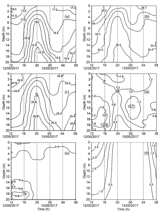
3.1 Hydrological conditions(Figs. 3 and 4) At 12 and 16 h, the upper layer(top 6 m)was heated by the solar radiation forming a certain gradient of water temperature(18. 5Ȃ17. 0 ℃). The water column condition changed at 20 h, due to the intrusion of colder(15.5Ȃ13.5 ℃)and saltier(34.4Ȃ34.6)water from the bottom during the flood. This intrusion mixed vertically the wa-ter column but was not strong enough to break the stratification up to the upper layer, forming a shallow layer thermocline at 1Ȃ6 m depth. At 00 h, when the water intrusion of the flood tide moved downward, and a thermocline was found at a deeper depth, 16Ȃ19 m with a temperature gradient(15.5Ȃ14.0 ℃).At 04 h, the water col-umn was well-mixed due to the high tidal cur-rent, and the colder and saltier water layer was located even deeper and almost not visible in our
Fig. 2 Tide level(m)during the survey at
Ta-teyama Bay, Japan. Bars represent start and end times of the samplings.
Fig. 3 Temporal changes in the vertical distribution of environmental properties on 12Ȃ13 May
2017.(a)water temperature(℃),(b)salinity,(c)sigma-t,(d)Chl-a(µg LȂ1),(e)turbidity (FTU),and(f)light intensity(PAR in log10µmol photons mȂ2sȂ1).
profiles. Later, at 08 h, the flood lifted this water mass again upwards, reaching the 16 m depth. At this time, the upper layer(0Ȃ14 m)remained well-mixed, showing a more homogeneous distri-bution of environmental parameters(Figs. 3a, b). The density profile showed the similar fluctua-tions governed by the temperature and salinity (Fig. 3c).
Regarding the chlorophyll-a fluorescence(Chl-a), the colder and saltier water found in the deeper layer that moved upwards during high tide showed distinctively low Chl-a(0.2Ȃ0.8 µg L-1).Above this pool, typical peaks of Chl-a(1.6 and 3.1 µg L-1)were observed at the bottom 18 m at 12 and 16 h, but at 20 h, peak(1.8 µg L-1) moved to the upper layer 2.5 m, coincided with a thermocline, and then moved back to the deeper depth 11.5 m at 00 h, and disappeared in 04 and 08 h, respectively(Fig. 3d).Water turbidity was higher at 12 and 16 h, especially in the bottom layers where a significant increase in the Chl-a was noticed(Fig. 3e). The values of 1% I0 depths(which indicate the bottom of the eu-photic layer)in the day-time samplings were 18 m at 12 h, 17 m at 16 h and 12 m at 08 h,
respec-tively(Figs. 3f and 4).
3.2 Spatial and temporal distributions of total phytoplankton(Fig. 5)
At 12 h, phytoplankton distribution was heter-ogeneous with high densities 134 ± 13 cells mL-1(mean ± standard deviation)in the up-per 0Ȃ4 m, and 115 ± 20 cells mL-1at 7.5Ȃ20 m, respectively, and a low density 72 ± 26 cells mL-1in the thermocline 4.5Ȃ7 m(Fig. 5a).At 16 h, phytoplankton showed a similar distribution pattern to that observed at 12 h, with high densi-ty 100 ± 13 cells mL-1in the upper 4 m but de-creased to 70 ± 9 cells mL-1in the thermocline (4.5Ȃ7 m)and again an increasing trend 90 ± 19 cells mL-1was observed below 7 m towards the bottom 20 m(Fig. 5b).Phytoplankton distribu-tion pattern totally changed at 20 h, which was characterized by the formation of the pro-nounced thermocline at a shallow depth(1Ȃ6 m), where phytoplankton were concentrated 61 ± 21 cells mL-1, but the distribution was restrict-ed below the thermocline(Fig. 5c). At 00 h, thermal stratification in the upper layer was not seen, but it appeared in a deeper layer(16Ȃ19 m).At that time, phytoplankton were abundant (76 ± 11 cells mL-1)above the thermocline at 9Ȃ14 m(Fig. 5d)and significantly decreased in the thermocline. The next samplings at 04 and 08 h, phytoplankton showed a rather homogene-ous vertical distribution pattern in the water col-umn(Figs. 5e, f),correspond with the effects of tidal mixing.
3.3 Phytoplankton assemblage composition (Table 1)
In our survey, a total of 22 phytoplankton taxa were identified, including 9 diatoms(Bacillario-phyceae)such as Thalassiosira sp.(3,520 cells mL-1, 27.5%),Dactyliosolen fragilissimus(1,776 cells mL-1, 13. 9%), Pseudo-nitzschia sp.(927
Fig. 4 Temporal changes in the vertical
distribu-tion of relative light intensity during 12Ȃ13 May 2017.
cells mL-1, 7. 2%), Coscinodiscus sp.(183 cells mL-1, 1.4%), Pleurosigma sp.(49 cells mL-1, 0.4%),Lauderia annulata(37 cells mL-1, 0.3%), Rhizosolenia setigera(17 cells mL-1, 0. 1%), Thalassionema nitzschioides(13 cells mL-1, 0.1%),and Meuniera membranacea(6 cells mL-1, 0.05%);10 dinoflagellates(Dinophyceae)such as Prorocentrum minimum(2, 622 cells mL-1, 20.5%),Scrippsiella trochoidea(1,612 cells mL-1,
12. 6%), Gyrodinium spirale(501 cells mL-1, 3.9%), Protoperidinium quinquecorne(253 cells mL-1, 2. 0%), Heterocapsa sp.(177 cells mL-1, 1.4%), Oxyphysis oxytoxoides(76 cells mL-1, 0.6%),Ceratium furca(23 cells mL-1, 0.2%),C. fusus(7 cells mL-1, 0.05%), Gonyaulax spinifera (10 cells mL-1, 0.1%), and Alexandrium sp.(7 cells mL-1, 0.05%);and other groups such as Ra-phidophyceae, Dictyochophyceae and
Haptophy-Fig. 5 Vertical distribution of total phytoplankton abundance for the six sampling times. Black
line: average phytoplankton abundance, with standard deviation bar from the triplicate counts. Grey line: Chl-a concentration.
ceae with only one species of each, Heterosigma akashiwo(303 cells mL-1, 2.4%),Dictyocha spec-ulum(10 cells mL-1, 0.1%),and Coccolithophor-id(468 cells mL-1, 3.7%), respectively, and un-identified phytoplankton(205 cells mL-1, 1.5%). Hence, the phytoplankton community was main-ly dominated by diatoms and dinoflagellates(50%
and 42% of the total cell density).
Specifically, among these species, Thalassio-sira sp., D. fragilissimus, Pseudo-nitzschia sp., P. minimum, and S. trochoidea were noted as the dominant species, which altogether contributed more than 80% of the total abundance of phyto-plankton. Therefore, we consider their
species-Table 1. List of phytoplankton in Tateyama Bay with total abundance,
per-centage, and average size(length and width).
Species Total abundance (µm)Length (µm)Width cells mLȂ1 % Bacillariophyceae Coscinodiscus sp. 183 1.4 50.0 37.7 Dactyliosolen fragilissimus 1,776 13.9 23.0 12.0 Lauderia annulata 37 0.3 23.7 16.9 Meuniera membranacea 6 0.05 57.8 31.1 Pleurosigma sp. 49 0.4 150.6 20.2 Pseudo-nitzschia sp. 927 7.2 30.3 4.6 Rhizosolenia setigera 17 0.1 379.0 5.2 Thalassionema nitzschioides 13 0.1 25.0 2.9 Thalassiosira sp. 3,520 27.5 18.9 12.5 Dinophyceae Alexandrium sp. 7 0.05 39.1 35.2 Ceratium furca 23 0.2 153.6 34.2 Ceratium fusus 7 0.05 343.7 30.5 Gonyaulax spinifera 10 0.1 29.6 23.1 Gyrodinium spirale 501 3.9 60.9 36.8 Heterocapsa sp. 177 1.4 30.7 21.1 Oxyphysis oxytoxoides 76 0.6 56.9 19.4 Prorocentrum minimum 2,622 20.5 22.2 18.5 Protoperidinium quinquecorne 253 2.0 23.7 18.7 Scrippsiella trochoidea 1,612 12.6 29.1 23.1 Dictyochophyceae Dictyocha speculum 10 0.1 29.5 21.3 Haptophyceae Coccolithophorid 468 3.7 13.2 12.3 Raphidophyceae Heterosigma akashiwo 303 2.4 29.8 24.3 Unidentified phytoplankton 205 1.5 13.9 11.9
specific distribution patterns in detail. The other species such as L. annulata, Coscinodiscus sp., Rhizosolenia sp., T. nitzschioides, M. membrana-cea, Pleurosigma sp., G. spirale, Alexandrium sp., G. spinifera, and Heterocapsa sp. were not ob-served in the colder and saltier water. Some dominant phytoplankton and the additional five species, P. quinquecorne, O. oxytoxoides, C. furca, C. fusus, and D. speculum that appeared after the high tide, only occurred in the colder and saltier water.
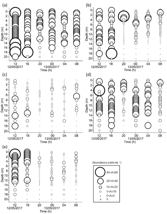
3.4 Species-specific distributions of dominant phytoplankton species(Fig. 6)
Thalassiosira sp. was numerically dominant throughout the study period and found at all sampling depths and times(Fig. 6a).D. fragilis-simus distribution coincided with the thermo-cline, and they were trapped in the thermocline (1Ȃ6 m)at 20 h by the strong density gradients. Moreover, the cell density decreased to approxi-mately the half(50%)after the high tide(18:20) and was not observed in the colder and saltier water mass(Fig. 6b).Pseudo-nitzschia sp. distri-bution pattern was not clear due to its low cell density throughout the sampling period(Fig. 6c).Similarly to Thalassiosira sp., P. minimum was detected at all sampling depths and times. An exception occurred at 20 h when a strong thermocline was marked at 1Ȃ6 m depth, where high cell densities were observed, but the distri-bution was limited below the thermocline(Fig. 6d).S. trochoidea distributed mainly in the first two samplings at 12 and 16 h; however, its distri-bution completely changed, and the abundance decreased to three-fourths(75%)after the high tide, 18:20(Fig. 6e).
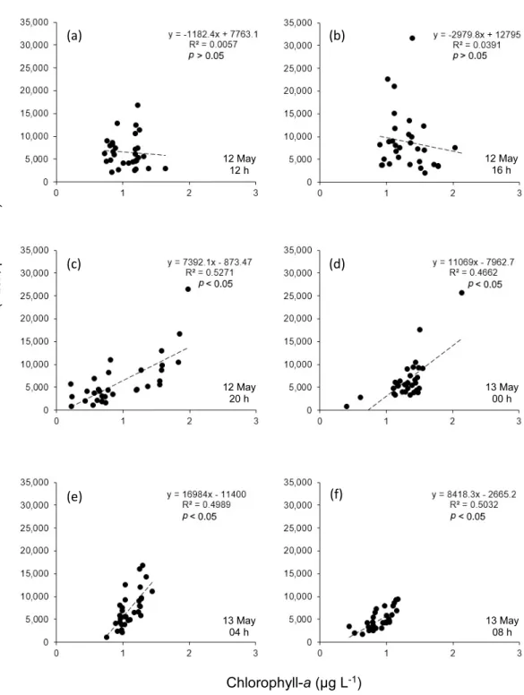
3.5 Phytoplankton biovolume versus Chl-a (Fig. 7)
At 12 and 16 h, the slope of the regression line
showed a negative correlation(p > 0.05),and an inverse relationship between the Chl-a and phy-toplankton biovolume was observed(Figs. 7a, b). Thus, relatively low phytoplankton biovolume was found at a depth of Chl-a peak 18 m, where small-sized diatom, Thalassiosira sp.(Table 1) was dominant in those samples. At 20 h, a statis-tically positive correlation(p < 0.05)was seen between the Chl-a and biovolume. At that time, Chl-a peak occurred in the upper layer(1Ȃ6 m), where higher phytoplankton biovolume was ob-served(Fig. 7c).In the following sample at 00 h, Chl-a and biovolume showed a positive correla-tion due to the occurrence of large-sized dinofla-gellates above the thermocline(9Ȃ14 m)where the Chl-a peak was detected(Fig. 7d). A posi-tive relationship was detected between the Chl-a Chl-and biovolume for 04 Chl-and 08 h, respectively (Figs. 7e, f).
An allometric relationship of Chl-a with biovo-lume was found in most sampling times except for 12 and 16 h. At these times, the Chl-a peak was observed at the bottom layer where higher turbidity was recorded.
3.6 Vertical distribution of aggregate parti-cles(Fig. 8)
Aggregates were generally more abundant in the first two samplings at 12 and 16 h(before high tide),especially at the bottom layers, with higher turbidity. After high tide(18:20),the for-mation of high abundance was not observed at the bottom in the following samplings at 20, 00, 04 and 08 h.
4. Discussion
Short-term phytoplankton dynamics are relat-ed to the changes of the water masses and hy-drodynamic gradients such as stratification and mixing processes, influenced by the periodic os-cillations of the tidal currents(BLAUW et al.,
Fig. 6 Vertical distribution of dominant phytoplankton species(average of the six samplings):(a)
Thalassiosira sp.,(b)Dactyliosolen fragilissimus,(c)Pseudo-nitzschia sp.,(d)Prorocentrum minimum, and(e)Scrippsiella trochoidea. “A” in the explanatory box represents “Abundance.”
Fig. 7 Relationship between Chl-a and FlowCAM biovolume of total phytoplankton from the cell counts
for 32 distinct vertical water layers(n = 32)during six sampling times.(a),(b),and(c)are for 12h, 16h, and 20h of 12 May;(d),(e),and(f)for 00h, 04h, and 08h of 13 May, respectively. The dashed line is fitted regression line.
2012).During our study period, thermal stratifi-cation was likely to be influencing the spatial heterogeneity of phytoplankton distribution. Stratification was pronounced under weak tidal mixing condition. Temperature gradients then divided the water column into different strata by the density gradients that restricted the phyto-plankton(but not entirely inhibit),resulting in a heterogeneous distribution. In contrast, it is like-ly that the vertical mixing generated by the tidal current homogenized the phytoplankton distri-bution in the water column. However, if tidal mixing was not strong enough, the water column could not be fully mixed, and stratification would remain in the upper layer. Thus, phytoplankton and Chl-a distributions differed among depths and sampling times due to the changes of the water masses and thermal structure.
In our study, both diatoms and dinoflagellates dominated the phytoplankton community. How-ever, their composition to the phytoplankton community was different in the different layers and times, related with the changes of the water
mass structure, and probably the thickness of the euphotic layer. Changes were pronounced in the day-time at 12 and 16 h, when stratification of water mass force to form the diatoms and di-noflagellates aggregation in the water column. At these times, a large proportion of diatoms contributed to the phytoplankton community near the bottom where a high value of Chl-a was observed(Fig. 9a). In contrast, dinoflagellates were detected mainly in the upper water column coinciding with the thermocline but rarely ob-served in the deeper parts of the euphotic zone (Fig. 9b).This might be because the dinoflagel-lates prefer stratified water mass as has been ex-plained in classical literatures(e.g. SMAYDA and REYNOLDS,2001).
Thalassiosira sp. and P. minimum occurred at all sampling depths and times. These are euryha-line and eurythermal species, that are common in temperate coastal environments(POPOVICH and GAYOSO, 1999; HAJDU et al., 2005). However, D. fragilissimus and S. trochoidea significantly decreased their abundance after the high tide,
Fig. 8 Vertical distribution of aggregate abundance(average value of the
triplicate analysis)for six sampling times. “A” in the explanatory box represents “Abundance.”
perhaps due to the changes of the water mass. During our survey, most phytoplankton species suddenly disappeared(except some dominant phytoplankton)after the high tide, when colder and saltier water mass intruded. It is suggested that these clear changes in species composition probably related to the changes of the water mass. Additionally, only five phytoplankton spe-cies, P. quinquecorne, O. oxytoxoides, C. furca, C. fusus, and D. speculum occurred in the colder and saltier water. Some of these five species(C. furca and C. fusus: Type VI(Coastal Entrained
Taxa))were noted as the coastal habitat (SMAYDAand REYNOLDS, 2001).
Regarding the phytoplankton biovolume and Chl-a, a significant positive correlation was found in most sampling times except for 12 and 16 h. At these exceptional times, discrepancies were apparent because of the relatively low phyto-plankton biovolume at a depth of Chl-a peak. In the case of 12 and 16 h, the water column was marked with a thermocline at 4. 5Ȃ7 m depth, which may act as a barrier(SPRINTALL and CRONIN, 2001)between the upper and lower
lay-Fig. 9 Vertical distribution of(a): diatoms and(b): dinoflagellates
abun-dance(average value of the triplicate analysis)for six sampling times. “A” in the explanatory box represents “Abundance.”
er. In the present study, the phytoplankton com-munity in the lower layer was dominated by the smaller size phytoplankton species, such as Tha-lassiosira sp. and D. fragilissimus. Thus, phyto-plankton biovolume was higher in the upper lay-er than those at a depth of Chl-a peak. Hence, a question rises “why Chl-a was high near the bot-tom?” We here speculate that the turbidity may be the key to answer this question because high-er turbidity values coincided with the bottom Chl-a peaks. MATSUIKEet al.(1986)reported the increase of suspended particles in the water col-umn is the major cause of water turbidity. This condition of high particle concentration leads to promote particle aggregation by colliding of smaller particles(JACKSON, 1990)or the release of phytoplankton structural bodies(ARMBRECHT et al., 2004),or together with sediments, and de-tritus(ZIMMERMANN-TIMM, 2002).
Our vertical profile of the aggregates showed that the particle densities were higher in the bot-tom at 12 and 16 h, where the highly turbid wa-ter mass was observed. However, it was gone af-ter the high tide, probably due to the intrusion of low turbidity water. At the same time, the Chl-a peak at the bottom disappeared, suggesting the relationship between the Chl-a and aggregate
particles. Hence, an additional experiment was done for the fluorescence analysis of the aggre-gates. Unfortunately, our formalin-fixed samples could not be used in the experiment, and thus we collected the fresh samples from the bottom water of Tokyo Bay while plankton survey cruis-ing at the inner Tokyo Bay. From our observa-tion with an epi-fluorescence microscope, emis-sion of fluorescence was detected from the aggregates(Figs. 10a, b).This finding provides additional evidence for the consideration of Chl-a concentrChl-ation in TChl-ateyChl-amChl-a BChl-ay, which shows the high value at the bottom is not only from the phytoplankton but also from the fluorescence due to the pigments deposited in the aggregate particles that were floating there.
5. Conclusions
To assess the fine-scale spatio-temporal phyto-plankton dynamics over a short time period, we used FlowCAM which can rapidly count, identi-fy and size the phytoplankton. Our results indi-cated that phytoplankton distribution changed significantly in a short timescale(such as sever-al hours)and in a few meters in depths, related with the eco-physiological characteristics of phy-toplankton, the stratification and vertical mixing. Therefore, studies based on monthly or seasonal survey of phytoplankton with depth-averaged samplings may not well reveal the real communi-ty structure and the distribution patterns of phy-toplankton that vary within a short time. Fur-thermore, our results showed that “Chl-a” does not always represent the phytoplankton abun-dance because it can be affected by detrital ag-gregate particles that contain a significant amount of fluorescent substances.
Acknowledgments
We thank the Laboratory of Aquatic Science Consultant Co., Ltd., which provided the use of a
Fig. 10 Images of aggregates captured by an
epi-fluorescence microscope using a fresh bottom sample obtained from Tokyo Bay as a trial.(a): bright field of aggregates,(b):fluorescence emits from aggregate under the dark field.
FlowCAM and lab facilities. Sincere thanks are to the captain and crew members of T/R/V Seiyo-maru and students of Plankton Laboratory of Tokyo University of Marine Science and Technology, who helped the field sampling of significant difficulties. The present work was partially supported by the Monbukagakusho Scholarship for KKG., and also by JSPS KAKEN-HI Grant Numbers JP18H02263 for YT.
References
ÁLVAREZ, E., M. MOYANO, Á. LÓPEZ-URRUTIA, E. NOGUEIRAand R. SCHAREK(2014):Routine deter-mination of plankton community composition and size structure: a comparison between Flow-CAM and light microscopy. J. Plankton Res., 36, 170Ȃ184.
ARMBRECHT, L. H., V. SMETACEK, P. ASSMYand C. KLAAS (2004): Cell death and aggregate formation in the giant diatom Coscinodiscus wailesii(Gran & Angst, 1931).J. Exp. Mar. Biol. Ecol., 452, 31Ȃ39. BLAUW, A. N., E. BENINCÀ, R. W. P. M. LAANE, N.
GREENWOODand J. HUISMAN(2012):Dancing with the tides: fluctuations of coastal phytoplankton orchestrated by different oscillatory modes of the tidal cycle. PLoS ONE, 7, e49319Ȃe49319. CAMOYING, M. G. and A. T. YÑIGUEZ(2016):FlowCAM
optimization: Attaining good quality images for higher taxonomic classification resolution of nat-ural phytoplankton samples. Limnol. Oceanogr.: Methods, 14, 305Ȃ314.
CARON, D. A., B. STAUFFER, S. MOORTHI, A. SINGH, M. BATALIN, E. A. GRAHAM, M. HANSEN, W. J. KAISER, J. DAS, A. PEREIRA, A. DHARIWAL, B. ZHANG, C. OBERGand G. S. SUKHATME(2008):Macro-to fine-scale spatial and temporal distributions and dy-namics of phytoplankton and their environmen-tal driving forces in a small montane lake in southern California, USA Limnol. Oceanogr., 53, 2333Ȃ2349.
DEKSHENIEKS, M. M., P. L. DONAGHAY, J. M. SULLIVAN, J. E. B. RINES, T. R. OSBORNand M. S. TWARDOWSKI (2001):Temporal and spatial occurrence of thin phytoplankton layers in relation to physical
processes. Mar. Ecol. Prog. Ser., 223, 61Ȃ71. GAST, L., A. N. MOURA, M. C. P. VILAR, M. K. CORDEIRO
-ARAÚJOand M. C. BITTENCOURT-OLIVEIRA(2014): Vertical and temporal variation in phytoplank-ton assemblages correlated with environmental conditions in the Mundaú reservoir, semi-arid northeastern Brazil. Braz. J. Biol., 74, 93Ȃ102. GERVAIS, F., U. SIEDEL, B. HEILMANN, G. WEITHOFF, G.
HEISIG-GUNKEL and A. NICKLISCH(2003): Small-scale vertical distribution of phytoplankton, nu-trients and sulphide below the oxycline of a mes-otrophic lake. J. Plankton Res., 25, 273Ȃ278. HAJDU, S., S. PERTOLAand H. KUOSA
(2005):Prorocen-trum minimum(Dinophyceae)in the Baltic Sea: morphology, occurrence- a review. Harmful Al-gae, 4, 471Ȃ480.
HARRIS, R. P., L. FORTIERand R. K. YOUNG(1986):A large-volume pump system for studies of the vertical distribution of fish larvae under open sea conditions. J. Mar. Biol. Ass. U. K., 66, 845Ȃ 854.
ITOH, H., A. TACHIBANA, H. NOMURA, Y. TANAKA, T. FUROTA and T. ISHIMARU(2011): Vertical distri-bution of planktonic copepods in Tokyo Bay in summer. Plankton Benthos Res., 6, 129Ȃ134. JACKSON, G. A.(1990): A model of the formation of
marine algal flocs by physical coagulation proc-esses. Deep-Sea Res., 37, 1197Ȃ 1211.
JAPANMETEOROLOGICAL AGENCYWEBSITE(2017):http: //www.data.jma.go.jp/kaiyou/data/db/tide/suis an/pdf_hourly/2017/TT.pdf.
LUNVEN, M., J. F. GUILLAUD, A. YOUÉNOU, M. P. CRASSOUS, R. BERRIC, E. LE GALL, R. KÉROUEL, C. LABRYand A. AMINOT(2005):Nutrient and phy-toplankton distribution in the Loire River plume (Bay of Biscay, France)resolved by a new Fine Scale Sampler. Estuar. Coast. Shelf Sci., 65, 94Ȃ108.
MATSUIKE, K., T. MORINAGA and T. HIRAOKA(1986): Turbidity distributions in Tokyo Bay and move-ment of the turbid water. J. Tokyo Univ. Fish.,
73, 97Ȃ114.
MAZNAH, W. O. W., S. RAHMAH, C. C. LIM, W. P. LEE, K. FATEMA and M. M. ISA(2016): Effects of tidal events on the composition and distribution of
phytoplankton in Merbok river estuary Kedah, Malaysia. Trop. Ecol., 57, 213Ȃ229.
MELLARD, J. P., K. YOSHIYAMA, E. LITCHMAN and C. A. KLAUSMEIER(2011): The vertical distribution of phytoplankton in stratified water columns. J. Theor. Biol., 269, 16Ȃ30.
POPOVICH, C. A. and A. M. GAYOSO(1999):Effect of ir-radiance and temperature on the growth rate of Thalassiosira curviseriata Takano(Bacillario-phyceae),a bloom diatom in Bahía Blanca estu-ary(Argentina).J. Plankton Res., 21, 1101Ȃ1110. POULTON, N. J. and J. L. MARTIN(2010):Imaging flow cytometry for quantitative phytoplankton analy-sis - FlowCAM. In Microscopic and Molecular Methods for Quantitative Phytoplankton Analy-sis. KARLSON, B., C. CUSACKand E. BRESNAN(eds.), UNESCO(IOC Manuals and Guides, no. 55.), Paris, p. 47Ȃ54.
SEE, J. H., L. CAMPBELL, T. L. RICHARDSON, J. L. PINCKNEY and R. SHEN(2005): Combining new technolo-gies for determination of phytoplankton com-munity structure in the northern Gulf of Mexico. J. Phycol., 41, 305Ȃ310.
SIERACKI, C. K., M. E. SIERACKI and C. S. YENTSCH (1998):An imaging in-flow system for automat-ed analysis of marine microplankton. Mar. Ecol. Prog. Ser., 168, 285Ȃ296.
SMAYDA, T. J. and C. S. REYNOLDS(2001):Community assembly in marine phytoplankton: application of recent models to harmful dinoflagellate blooms. J. Plankton Res., 23, 447Ȃ461.
SPRINTALL, J. and M. F. CRONIN(2001):Upper ocean vertical structure. In Encyclopedia of Ocean Sci-ence. STEELE, J. H., S. A. THORPE and K. K. TUREKIAN(eds.),Academic Press, San Diego, p. 3120Ȃ3129.
TAUXE, L., J. L. STEINDORFand A. HARRIS (2006):Dep-ositional remanent magnetization: Toward an improved theoretical and experimental founda-tion. Earth Planet. Sci. Lett., 244, 515Ȃ529. TILZER, M. M. and C. R. GOLDMAN(1978):Importance
of mixing, thermal stratification and light adap-tation for phytoplankton in Lake Tahoe(Cali-fornia, Nevada).Ecology, 59, 810Ȃ821.
ZIMMERMANN-TIMM, H.(2002): Characteristics,
dynamics and importance of aggregates in rivers -An invited review. Int. Rev. Hydrobiol., 87, 197Ȃ240.
Received: 26 April, 2019 Accepted: 6 August, 2019