Vol. 55, No. 1, March 2012, pp. 63–72
RELAXED DIVISOR METHODS AND THEIR SEAT BIASES
Tetsuo Ichimori
Osaka Institute of Technology
(Received October 26, 2010)
Abstract A class of methods of apportionment called the relaxed divisor methods is introduced here. It is theoretically shown that their biases between small and large states decrease and eventually approach zero as the house size increases. Because the methods of Hill and Webster are examples of the class, they both are practically unbiased for the house size large enough. However, computer simulations performed here strongly suggest that Webster is the first method to practically attain a state of unbiasedness when the house size increases from 200 to 43,500.
Keywords: Discrete optimization, apportionment, divisor methods, seat bias
1. Introduction
The apportionment problem is defined by Article I, Section 2 of the U.S. Constitution, which requires that seats of representatives shall be apportioned among the states, based proportionally on their population. Because seats are not dividable, it is impossible to com-pletely satisfy the constitutional requirement and some deviation from strict proportionality is unavoidable. This fact leads to a long debate over 200 years.
In the history of apportionment, the discovery of the Alabama paradox∗ was a terrible blow to Congress and it became urgent to seek apportionment methods not subject to the paradox. Huntington [6] discovered that his pairwise comparison approach yields the so-called “five historical methods” which avoid the paradox. They are the methods of Adams, Dean, Hill, Webster and Jefferson which already appeared in the history of apportionment. Because long years of experience showed that these methods favor small states in this order, he claimed that the Hill method stands in the middle of these five methods with respect to bias, namely, it does not favor small states or large states. His claim was reinforced by a National Academy of Sciences committee in 1929, and later again in 1948. On the other hand, around the same time as Huntington, Willcox [14] paid careful attention to empirical data and claimed that the Webster method best secures the end of holding balance between small and large states.
After several decades Balinski and Young [3] showed that there are an infinity number of methods of apportionment, called the divisor methods which avoid the population paradox† and they claimed that the Webster method exists in the middle of all divisor methods with respect to bias, while the Hill method is consistently biased toward small states. Note that any method not subject to the population paradox avoids the Alabama paradox.
∗A peculiar phenomenon that an increase in the number of seats causes a state to lose a seat. After the 1880 census it was reported to Congress that 8 seats would have assigned to Alabama with a house size of 299, while 7 seats with a house size of 300.
†Another peculiar phenomenon that a state with greater growth in population can lose a seat to a state with less growth.
Regarding the case of United States Department of Commerce v. Montana, 503 U.S. 442 (1992), Ernst [5] claimed that the Webster method is biased in favor of large states and the Hill method is unbiased in his sense.
Recently Drton and Schwingenschl¨ogl [4] have showed rather rigorously that the Webster method is asymptotically unbiased as the house size tends to infinity. Schuster et al. [10] have observed that the Webster method produces practically unbiased apportionments under the 1960–2000 censuses. On the other hand, they have observed that the Hill method also produces practically unbiased apportionments under the 1960–2000 censuses.
In light of these circumstances it would be imperative to decide which method is unbi-ased, Hill’s or Webster’s method. For this purpose a subclass of the divisor methods called “the relaxed divisor methods” are developed in Section 2. They are all theoretically shown to be more unbiased as the house size becomes large in Section 3. Because the methods of Hill and Webster are members of this subclass, both are practically unbiased for the house size large enough.
In Section 4 it is investigated by executing computer simulations how biased they are as the house size increases. As a result, it is confirmed that the relaxed divisor methods are more unbiased as the house size becomes large, while the methods of Adams and Jefferson which are not relaxed divisor methods are consistently biased to small states and to large states, respectively. In addition, these simulations show that Webster is the first method to practically attain a state of unbiasedness.
2. Apportionment Methods
In this section, first, the definition of the divisor methods is given. Then the relaxedly proportional methods developed by the author [8] are briefly described. The methods of Hamilton, Hill and Webster are examples of the relaxedly proportional methods. Finally, the relaxed divisor methods are proposed.
2.1. Divisor methods
Let N and N+ denote the sets of non-negative integers and positive integers, respectively.
Define a real valued function d(a) for a ∈ N, known as a rounding criterion. The function
d(a) is strictly increasing in a. It satisfies a≤ d(a) ≤ a + 1 for a ∈ N and moreover satisfies d(b) = b and d(c) = c + 1 for no pair of integers b∈ N+ and c∈ N.
Let z be a positive real number and let [z] denote an integer defined by the following rule:
1. If z < d(0), then [z] = 0.
2. If d(a) < z < d(a + 1) for some a∈ N, then [z] = a + 1. 3. If z = d(a) for some a∈ N, then [z] = a or a + 1.
Next, let M denote a divisor method and x > 0 be a divisor. A divisor x means that each seat is given an approximate constituency of x persons. Let s denote the number of states and h ≥ s the house size, i.e., the total number of seats; the values s = 50 and
h = 435 are of practical interest. Let pi > 0 denote the population of state i. If the equality
∑s
i=1[pi/x] = h is achieved for some divisor x > 0, then the number of seats to which
state i is entitled is ai = [pi/x]; pi/x is referred to as the “quotient” of state i and the
s-vector a = (a2, a2, . . . , as) an “apportionment” of h. Given p = (p1, p2, . . . , ps), h ≥ s,
and d(a), a∈ N, a divisor method M is defined as the set of apportionments [2]: { a ai = [p i x ] and s ∑ i=1 [p i x ] = h for some x > 0 } .
Although there can be an infinite numbers of divisor methods, the following five historical methods have received special treatment for a long time:
• the Adams method defined with d(a) = a,
• the Dean method defined with d(a) = a(a + 1)/(a + 0.5), • the Hill method defined with d(a) =√a(a + 1),
• the Webster method defined with d(a) = a + 0.5, • the Jefferson method defined with d(a + 1) = a + 1. 2.2. Relaxedly proportional methods
Let the set of states be denoted by S = {1, 2, . . . , s} and define v(S) = ∑si=1vi for any
s-tuple (v1, v2, . . . , vs). Let R+ denote the set of positive real numbers and let “s.t.” be an
abbreviation for “subject to” throughout this article.
Most of reasonable apportionment methods have their equivalent discrete optimization problems. For example, the Webster method has the following equivalent discrete optimiza-tion problem: PW min s ∑ i=1 a2 i pi
s.t. a(S) = h and ai ∈ N for i ∈ S.
Let W denote the set of all optimal solutions a = (a1, . . . , as) to the above problem PW,
then it is well known that W defines the Webster method, see [3]. In other words, any apportionment of h produced by the Webster method minimizes ∑ia2
i/pi subject to the
above constraints, while any optimal solution a = (a1, . . . , as) to the above problem PW is
an apportionment of h under the Webster method. Next consider its continuous relaxation:
min s ∑ i=1 a2 i pi
s.t. a(S) = h and ai ∈ R+ for i∈ S.
Then it is clear that there can exist some positive λ > 0 such that d(a2
i/pi)/dai = 2(ai/pi) =
λ for any i∈ S at optimality, which means that ai is completely proportional to pi for any
i at optimality. In other words, ai = (λ/2)pi = (h/p)pi = qi at optimality, where p denotes
the total population, i.e., p = ∑pi and qi = (h/p)pi is called the “quota” of state i, i.e.,
the ideal share of state i. Then, the Webster method is said to be “relaxedly proportional.” In general, if an apportionment method has its equivalent discrete optimization problem and its continuous relaxation has an optimal solution identical to the vector of quotas, i.e.,
a = q, then the method is defined to be relaxedly proportional.
Similarly, the Hill method has the following equivalent discrete optimization:
min s ∑ i=1 p2 i ai
s.t. a(S) = h and ai ∈ N+ for i∈ S.
Since its continuous relaxation is: min s ∑ i=1 p2i ai
s.t. a(S) = h and ai ∈ R+ for i∈ S,
On the other hand, the methods of Adams, Dean and Jefferson are not relaxedly propor-tional. For example, the Adams method has the following equivalent discrete optimization [7]: min s ∑ i=1 a2i − ai pi
s.t. a(S) = h and ai ∈ N for i ∈ S.
Its continuous relaxation has an optimal solution ai = λpi + 0.5 where λ = (h− s/2)/p.
This means that ai is not proportional to pi. Since the term 0.5 has a great influence on
small states, the Adams method favors small states in this sense. Similarly, the Jefferson method minimizes ∑i(a2
i + ai)/pi and an optimal solution to its continuous relaxation is
ai = λpi− 0.5 where λ = (h + s/2)/p. Hence it favors large states in this sense.
Although there are an infinite numbers of the relaxedly proportional methods, the fol-lowing three methods along with Hill’s and Webster’s methods are considered here. The first one was developed by Theil and Schrage [13]. The second one was proposed by Theil [12]. The last one was suggested by this author [8]. In fact, the first two have been rediscovered by Agnew [1] recently.
• The Theil-Schrage method defined with d(0) = 0 and d(a) = 1/ log((a+1)/a) for a ∈ N+
has its equivalent optimization:
min
s
∑
i=1
(−pilog ai) s.t. a(S) = h and ai ∈ N+ for i∈ S.
• The Theil method defined with d(0) = 1/e ≈ 0.37 and d(a) = (1/e)(a + 1)a+1/aa for
a∈ N+ has its equivalent optimization:
min s ∑ i=1 ailog ai pi
s.t. a(S) = h and ai ∈ N for i ∈ S.
• The “1/3” method defined with d(a) = √a2+ a + 1/3 for a ∈ N has its equivalent
optimization: min s ∑ i=1 a3 i p2 i
s.t. a(S) = h and ai ∈ N for i ∈ S.
It is easy to show that these three are relaxedly proportional. Instead of the five historical methods, define the “new five,” namely, the methods of Hill, Theil-Schrage (T&S for short), Theil, Webster and “1/3” in order to compare mainly Hill’s and Webster’s methods.
2.3. Relaxed divisor methods
The relationship between the new five methods and their respective equivalent discrete optimization problems can be easily generalized. For convenience, define 1/0 = +∞, log 0 =
−∞ and R = {x | −∞ < x < +∞}, where it should be noted that infinities ±∞ are not
included in R in a customary way.
Consider the following discrete optimization for a finite real number n ∈ R :
P: min
a s
∑
i=1
where f (ai, pi) = ailog ai pi if n = 0 −pilog ai if n =−1 an+1i n(n + 1)pn i otherwise. (2.1)
Although f (ai, pi) seems to be a function of “two variables” ai and pi, consider f (ai, pi) a
function of one variable ai because pi is a constant. Notice that n = 0 corresponds to Theil,
n =−1 to T&S, n = 2 to “1/3,” n = −2 to Hill and n = 1 to Webster.
Consider the difference f (ai+ 1, pi)− f(ai, pi), then it can be written as follows:
f (ai+ 1, pi)− f(ai, pi) = log (ai+ 1) ai+1 aai i pi if n = 0 pilog ai ai+ 1 if n = −1 (ai+ 1)n+1− an+1i n(n + 1)pn i otherwise. (2.2)
Next, define the function d(a), a∈ N+ (as a rounding criterion‡) as follows:
d(a) = lim n→0 ( (a + 1)n+1− an+1 n + 1 )1 n = 1 e (a + 1)a+1 aa if n = 0 lim n→−1 ( (a + 1)n+1− an+1 n + 1 )1 n = 1 loga+1a if n = −1 ( (a + 1)n+1− an+1 n + 1 )1 n otherwise. (2.3)
And define d(0) as follows:
d(0) = 0 if n≤ −1 1 e ≈ 0.37 if n = 0 1 n √ n + 1 otherwise. (2.4)
For d(a) defined in (2.3) it is shown in [11] that a < d(a) < a + 1 when n is finite. Because the values of d(a) relate intimately with the (relative but not absolute) biases of apportionment methods (see [9] for details), it is important to note that the function d(a) in (2.3) is strictly increasing in n for each fixed positive a ∈ N+. In addition, d(0) is also
strictly increasing in n >−1 while d(0) = 0 for n ≤ −1.
Recall here the definition of a divisor method M . It is shown in [3] that M is equivalent
to { a max ai>0 d(ai − 1) pi ≤ min aj≥0 d(aj) pj and a(S) = h } . (2.5)
‡Appearing in (2.3), the first (1/e)(a + 1)a+1/aa is the identric mean of two consecutive integers a≥ 1 and
Moreover, it can be easily shown that the following set: {
a a is optimal for problem P
} (2.6) is identical to { a max ai>0{f(a i, pi)− f(ai− 1, pi)} ≤ min aj≥0{f(a
j + 1, pj)− f(aj, pj)} and a(S) = h
}
, (2.7)
see Ibaraki and Katoh [7] for details.
Compare (2.2) and (2.3), then it follows from (2.5) and (2.7) that the set (2.6) defines a class of divisor methods with d(a) in (2.3). Let these divisor methods be referred to as the “relaxed divisor methods.” In fact, the relaxed divisor methods are relaxedly proportional, which will be shown below.
Theorem 2.1. The relaxed divisor methods are relaxedly proportional. Proof. The continuous relaxation of the problem P is
min
a s
∑
i=1
f (ai, pi) s.t. a(S) = h and ai ∈ R+ for i∈ S.
It is easy to find that an optimal solution is a = q because f′′(ai, pi) > 0 means that there
exist a λ satisfying f′(ai, pi) = λ for any i∈ S. Hence the theorem.
3. Absolute Biases of Relaxed Divisor Methods
Here absolute biases§ of the relaxed divisor methods are considered. For relative biases of methods of apportionment, see [3, 10].
Define the set B = {k/L | k ∈ N} for a positive integer L. Then consider the following “weak relaxation” of the problem P:
min
a s
∑
i=1
f (ai, pi) s.t. a(S) = h and ai ∈ B for i ∈ S.
In fact, it may be assumed that L is a rational if Lh is a positive integer. Let bi = Lai.
Then the relation a(S) = h is equivalent to b(S) = Lh. It is easy to obtain the followings:
s ∑ i=1 f (bi, pi) = L s ∑ i=1 ailog ai pi + (L log L)h if n = 0 −p(S) log L − s ∑ i=1 pilog ai if n =−1 Ln+1 s ∑ i=1 an+1i n(n + 1)pn i otherwise. (3.1)
Namely, the objective function∑si=1f (bi, pi) is expressed as s ∑ i=1 f (bi, pi) = C s ∑ i=1 f (ai, pi) + D
§Although virtually impossible, a method is absolutely unbiased if∑
where C is a positive constant and D is a constant. Since C is positive, this means that minimizing ∑si=1f (bi, pi) is equivalent to minimizing
∑s
i=1f (ai, pi). Hence the above weak
relaxation can be rewritten as: min b s ∑ i=1 f (bi, pi) s.t. b(S) = Lh and bi ∈ N for i ∈ S.
Theorem 3.1. The relaxed divisor methods are more unbiased as the house size becomes
large.
Proof. The relaxed divisor methods yield the apportionment completely proportional to the
population of states if the constraint ai ∈ N is relaxed to ai ∈ R+ for every i ∈ S. As the
integer L of the weak relaxation of P becomes large, the weak relaxation becomes closer to the continuous relaxation problem. Moreover, increasing of L implies the increase of the house size. Hence the theorem.
4. Simulation
In order to verify the theoretical result in the preceding section, some computer simulations are performed for the new five methods. There are a number of empirical tests for bias proposed by Balinski and Young [3], by Ernst [5], by Schuster et al. [10] and others. Although most of them depend on the differences |ai− qi|, the differences tend to be smaller as the
house size increases. In fact, if h = p where h is the house size and p is the total population, then most of reasonable methods produce unbiased apportionments, i.e., ai = pi for any
i∈ S. Therefore the differences |ai− qi| become zero. Because the simulations here use the
large house sizes, such tests seem not to fulfill our purpose.
Our bias test is as follows. Based on the population of states (p1, p2, . . . , ps), let an
apportionment (a1, a2, . . . , as) be produced by any method of apportionment. Define the
following sets: F = { (i, j) 1 ≤ ai < aj and ai pi > aj pj i, j ∈ S } and A = { (i, j) 1 ≤ ai < aj i, j ∈ S } .
Note that (i, j)∈ F means that the smaller state i is favored over the larger state j under any divisor method. Then the value|F |/|A| represents the bias ratio¶ that small states are favored [3].
First, according to the 2000 census fix an apportionment of the 435 seats among the 50 states produced by each of the new five methods. In fact, the Hill method produces the current apportionment. For each method M, let the fixed apportionment be denoted by
a(M ) and its divisor by x(M ), i.e., ai(M ) = [pi/x(M )] where pi is the population of state
i for the year 2000.
Let random Pi be uniformly distributed on the interval
d(ai(M )− 1)x(M) ≤ Pi ≤ d(ai(M ))x(M ),
then the apportionment produced by M based on the random populations P1, . . . , Ps is the
same as that based on the actual population according to the 2000 census.
To avoid the unrealistic assumption of very small states, assume in estimating the bias of M that no state’s quotient is less than 0.5. In other words, the random population of each state is assumed to be uniformly distributed on the interval
max{0.5, d(ai(M ))}x(M) ≤ Pi ≤ d(ai(M ))x(M ).
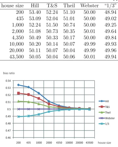
One million tuples of populations (P1, P2, . . . , Ps)’s are generated for each of the new five
methods and for each value of the house size h, where h takes values 200, 435, 1,000, 2,000, 4,350, 10,000, 20,000, and 43,500. Then the bias is estimated for each method and each h, see Table 1 and Figure 1. In addition, the same simulation is run for the 1990 census, see Table 2. It can be understood that the bias ratios of the new five methods converge to 50%, and that Webster is the first method to practically attain the 50% bias ratio. In fact, it keeps about 50% for any house size.
On the other hand, the methods of Adams and Jefferson show the consistent strong biases according to the same simulations as for the new five methods, see Table 3.
Table 1: Each entry denotes the average bias ratio (%) for one million tests applying one of the new five for each of various house sizes on the basis of the 2000 apportionment
house size Hill T&S Theil Webster “1/3” 200 53.40 52.24 51.10 50.00 48.94 435 53.09 52.04 51.01 50.00 49.02 1,000 52.24 51.50 50.74 50.00 49.25 2,000 51.08 50.73 50.35 50.01 49.64 4,350 50.49 50.33 50.17 50.00 49.84 10,000 50.20 50.14 50.07 49.99 49.93 20,000 50.11 50.07 50.04 49.99 49.96 43,500 50.05 50.04 50.06 50.01 49.94 0.46 0.47 0.48 0.49 0.5 0.51 0.52 0.53 0.54 200 435 1000 2000 4350 10000 20000 43500 Hill T&S Theil Webster 1/3 house size bias ratio
Figure 1: The house size h is placed on the horizontal axis and the bias ratio is on the vertical axis
5. Concluding Remarks
We showed in this paper that there can exist a subclass of the divisor methods whose biases decrease and eventually approach zero as the house size increases. They are called
Table 2: Each entry denotes the average bias ratio (%) for one million tests applying one of the new five for each of various house sizes on the basis of the 1990 apportionment
house size Hill T&S Theil Webster “1/3” 200 53.36 52.21 51.10 50.01 48.99 435 53.11 52.08 51.01 49.99 48.99 1,000 52.15 51.46 50.73 49.99 49.26 2,000 51.05 50.71 50.35 50.00 49.65 4,350 50.47 50.32 50.16 50.00 49.85 10,000 50.21 50.15 50.06 50.00 49.93 20,000 50.11 50.05 50.03 50.00 49.96 43,500 50.05 50.05 50.06 50.00 49.94
Table 3: Each entry denotes the average bias ratio (%) for one million tests applying one of the Adams and Jefferson methods for each of various house sizes on the basis of the 2000 apportionment
house size Adams Jefferson 200 73.20 18.46 435 78.36 17.86 1,000 79.35 18.91 2,000 79.44 19.80 4,350 79.52 20.14 10,000 79.54 20.37 20,000 79.41 20.48 43,500 79.41 20.56
the relaxed divisor methods and the methods of Hill and Webster are examples of them. Hence both of the two methods are practically unbiased when the house size is large enough. In other words, Huntington and Willcox are both right if the house size is large enough. However, if the house size is the current number of representatives, i.e., 435, then the simulations performed here strongly suggest that Willcox is right.
References
[1] R.A. Agnew: Optimal congressional apportionment. American Mathematical Monthly,
115 (2008), 297–303.
[2] M.L. Balinski: The problem with apportionment. Journal of the Operations Research
Society of Japan, 36 (1993), 134–148.
[3] M.L. Balinski and H.P. Young: Fair Representation (Yale University Press, New Haven, 1982).
[4] M. Drton and U. Schwingenschl¨ogl: Asymptotic seat bias formulas. Metrika, 62 (2005), 23–31.
[5] L.R. Ernst: Apportionment methods for the House of Representatives and the court challenges. Management Science, 40 (1994), 1207–1227.
[6] E.V. Huntington: The apportionment of representatives in Congress. Transactions of
[7] T. Ibaraki and N. Katoh: Resource Allocation Problems (MIT Press, Cambridge, 1988). [8] T. Ichimori: New apportionment methods and their quota property. JSIAM Letters, 2
(2010), 33–36.
[9] A.W. Marshall, I. Olkin, and F. Pukelsheim: A majorization comparison of apportion-ment methods in proportional representation. Social Choice and Welfare, 19 (2002), 885–900.
[10] K. Schuster, F. Pukelsheim, M. Drton, and N.R. Draper: Seat biases of apportionment methods for proportional representation. Electoral Studies, 22 (2003), 651–676.
[11] K.B. Stolarsky: Generalizations of the logarithmic mean. Mathematics Magazine, 48 (1975), 87–92.
[12] H. Theil: The desired political entropy. American Political Science Review, 63 (1969), 521–525.
[13] H. Theil and L. Schrage: The apportionment problem and the European Parliament.
European Economic Reviews, 9 (1977), 247–263.
[14] W.F. Willcox: The apportionment of representatives. American Economic Review, 6 Supplement (1916), 3–16.
Tetsuo Ichimori
Osaka Institute of Technology 1-79-1 Kitayama, Hirakata City Osaka 573-0196, Japan