The Automorphism Groups of Enriques
Surfaces Covered by Symmetric Quartic Surfaces
Dedicated to Prof. Robert Lazarsfeld on his 60th birthday
By
Shigeru MUKAI and Hisanori OHASHI
February 2014
R
ESEARCH
I
NSTITUTE FOR
M
ATHEMATICAL
S
CIENCES
SHIGERU MUKAI AND HISANORI OHASHI
Dedicated to Prof. Robert Lazarsfeld on his 60th birthday
Abstract. Let S be the (minimal) Enriques surface obtained from the symmetric quartic surface (Pi<jxixj)2 = kx1x2x3x4 inP3 with k 6=
0, 4, 36, by taking quotient of the Cremona action (xi)7→ (1/xi). The automorphism group of S is a semi-direct product of a free productF of four involutions and the symmetric group S4. Up to action ofF, there
are exactly 29 elliptic pencils on S.
The automorphism groups of very general Enriques surfaces, namely those corresponding to very general points in moduli, were computed in Barth-Peters[1] as an explicitly described infinite arithmetic group. Also many authors [3, 1, 9, 5] studied Enriques surfaces with only finitely many auto-morphisms. The article [1] also includes an example whose automorphism group is infinite but still virtually abelian group. In this paper we give a concrete example of an Enriques surface whose automorphism group is not virtually abelian. Moreover, the automorphism group is explicitly described in terms of generators and relations. See also Remark 5.
We work over any algebraically closed field whose characteristic is not two. Let us introduce the quartic surface with parameters k and l,
(1) X : {s22= ks4+ ls1s3} ⊂ P3,
where sd are the fundamental symmetric polynomials of degree d in the
homogeneous coordinates x1, . . . , x4. It is singular at the four coordinate points (1 : 0 : 0 : 0), . . . , (0 : 0 : 0 : 1) and has an action of the symmetric group S4. It also admits the action of the standard Cremona transformation
ε : (x1 :· · · : x4)7→ ( 1 x1 :· · · : 1 x4 )
which commutes with S4. After taking the minimal resolution X, the
quo-tient surface S = X/ε becomes an Enriques surface, whenever X avoids the eight fixed points (±1 : ±1 : ±1 : 1) of ε. This condition is equivalent to
k + 16l̸= 36, k ̸= 4 and 4l + k ̸= 0.
2000 Mathematics Subject Classification. 14J28, 20F55.
Supported in part by the JSPS Grant-in-Aid for Scientific Research (B) 22340007, (S) 19104001, (S) 22224001, (S)25220701, (A) 22244003, for Exploratory Research 20654004 and for Young Scientists (B) 23740010.
The projection from one of four coordinate points exhibits X as a double cover of the projective plane P2. The associated covering involution com-mutes with ε and defines an involution of the Enriques surface S. In this way we obtain four involutions σi (i = 1, . . . , 4). The action of S4 also descends
to S. Therefore, by mapping the generators of C2∗4 to σi, we obtain a group
homomorphism
(2) S4n (C2∗4)→ Aut(S),
where S4 acts on the free product as permutation of the four factors.
In this paper we study the automorphism group and elliptic fibrations of
S in the case l = 0. Our main result is as follows.
Theorem 1. (=Theorem 3.7) In the equation (1), let l = 0 and k̸= 0, 4, 36.
Then (2) is an isomorphism. Namely Aut(S) is isomorphic to the
semi-direct product of the free productF of four involutions σi (i = 1, . . . , 4) and
the symmetric group S4.
In the proof of this theorem, we also obtain the following results on elliptic pencils and smooth rational curves. Let S be as in Theorem 1.
Theorem 2. (= Theorem 3.4) Up to the action of the free productF ≅ C2∗4, there are exactly 29 elliptic pencils on S. They are classified into five types and the main properties are as in the following table.
singular fibers Mordell-Weil rank number
1) E7˜ + ˜A1 0 12
2) E6˜ + ˜A2 0 4
3) D6˜ + ˜A1 1 6
4) A7˜ + ˜A1 0 3
5) 2 ˜A5+ ˜A2+ ˜A1 0 4
Here 2 ˜Andenotes the multiple singular fiber of type ˜Anand the Mordell-Weil
rank stands for that of its Jacobian fibration.
Theorem 3. (= Theorem 3.3) Up to the action of the free productF ≅ C2∗4, there are exactly sixteen smooth rational curves on S. They are represented by the curves in the configuration 10A + 6B (see below).
The proof of Theorem 1 uses some sixteen smooth rational curves on S and the fact that four involutions σ1, . . . , σ4are numerically reflective. First
using the four singularities of type D4 and four tropes on X, we find ten
smooth rational curves on S with the dual graph as in Figure 1 (Section 1). We call it the 10A configuration.
Also by looking at some other plane sections, we find further six smooth rational curves on S with the dual graph as in Figure 2. This is called the 6B configuration.
We denote by N S(S)f the N´eron-Severi lattice of S modulo torsion. The
E2 E3 E1 E12 E 4 E14
Figure 1. The 10A configuration.
F23 F13
F12
F34
Figure 2. The 6B configuration
G1, . . . , G4 ∈ NS(S)f, respectively. For instance, the class G1 is E2+ E23+
E3+ E34+ E4+ E24− E1 in terms of Figure 1 (Proposition 2.1). The dual
graph of these four (−2) classes is the complete graph in four vertices with doubled edges. This is what is called the 4C configuration.
We can check that the twenty (−2)-classes Ei, Eij, Fij, Gi define a convex
polyhedron whose Coxeter diagram satisfies the Vinberg’s condition [12]. Namely the subgroup W (10A + 6B + 4C) generated by reflections in these twenty classes has finite index in the orthogonal group O(N S(S)f). In fact,
the limit of our Enriques surfaces as k → ∞ is of type V in Kondo[5] (see Remark 2.3), and our diagram coincides with Kondo’s. Although in his case the classes G1, . . . , G4 were also represented by smooth rational curves, in our case they appear just as the center of the reflective involutions σ1, . . . , σ4
and are not effective (Corollary 2.2).
To prove our Theorem 1, we divide the generators of W (10A + 6B + 4C) into two parts, those coming from 10A + 6B and those from 4C. By a lemma of Vinberg[11], W (10A + 6B + 4C) is the semi-direct product
W (4C)n N(W (10A + 6B)), where N denotes the normal closure. Since the
whole 10A + 6B + 4C configuration has only S4-symmetry, we obtain our
Theorem 1 and the others (Sections 3).
(1) When (k− 4)(l − 4) = 16, the surface X is Kummer’s quartic surface Km(J (C)) written in Hutchinson’s form. It has 16 nodes. Our four involu-tions σiare called projections. As is shown in [7], S is an Enriques surface of
Hutchinson-G¨opel type and the four involutions are numerically reflective. Especially in the case (k, l) = (−4, 2), the hyperelliptic curve C branches over the vertices of regular octahedron and the equation of X becomes
(x21x22+ x23x42) + (x21x23+ x22x24) + (x21x24+ x22x23) + 2x1x2x3x4 = 0.
This is the case of the octahedral Enriques surface [8] and S is isomorphic to the normalization of the singular sextic surface
x21+ x22+ x23+ x24+√−1 ( 1 x2 1 + 1 x2 2 + 1 x2 3 + 1 x2 4 ) x1x2x3x4= 0.
In these cases we know that there exist automorphisms on S induced from
X other than projections, namely some switches and correlations. The
au-tomorhism group of the octahedral Enriques surface will be discussed else-where.
(2) The quartic surface X : ks4+ ls1s3 = 0 is the Hessian of the cubic
surface
k(x31+ x32+ x33+ x43) + l(x1+ x2+ x3+ x4)3= 0.
The case (k : l) = (1 : −1) is most symmetric among this one-parameter family. In this special case, the Enriques surface S = X/ε is of type VI in Kondo[5] and the automorphism group is isomorphic to S5. In particular,
the homomorphism (2) is neither injective nor surjective.
Remark 5. In terms of virtual cohomological dimensions of discrete groups [10], our example can be located in the following way. The virtual cohomo-logical dimension is equal to 0 for finite groups. On the other extreme, the discrete group Aut(S) for very general Enriques surfaces S has the virtual cohomological dimension 8. See [2]. In our case, the automorphism group has virtual cohomological dimension 1.
1. Smooth rational curves Under the condition l = 0, the equation (1) becomes
(3) X : (x1x2+ x1x3+ x1x4+ x2x3+ x2x4+ x3x4)2 = kx1x2x3x4.
This surface has four rational double points of type D4at the four coordinate
points (1 : 0 : 0 : 0), . . . , (0 : 0 : 0 : 1) and by taking the quotient of the minimal resolution X by the standard Cremona involution
ε : (x1:· · · : x4)7→ ( 1 x1 :· · · : 1 x4 ) ,
we obtain an Enriques surface S = X/ε. We begin with the study of the configuration of smooth rational curves on the surfaces.
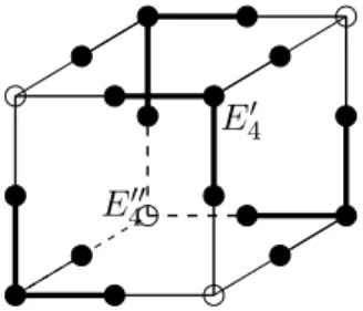
The desingularization X has sixteen smooth rational curves as the excep-tional curves of the four D4 singularities. Also each coordinate plane cuts
E4′′
E4′
Figure 3. The quartic surface with four D4 singularities.
the quartic doubly along a conic, which defines a smooth rational curve on
X. They are called tropes. The configuration of these twenty curves is as
in Figure 3, which depicts the dual graph. Black vertices come from the singularities and white ones are tropes.
The standard Cremona involution ε acts on Figure 3 by the point sym-metry. Therefore the Enriques surface S has ten smooth rational curves whose dual graph is the one in Figure 1. In what follows, we call these ten curves on S the 10A configuration. The indexing is given as follows. Since a vertex of the tetrahedron corresponds to two curves on X, namely the trope {xi = 0} and the central component of the exceptional curves at
(0 : · · · : 1 : · · · : 0) (the i-th coordinate is 1), we denote the curve at the
vertex by Ei (i = 1, . . . , 4). Also if a vertex at the middle of an edge is
connected to two vertices, say Ei and Ej, then we denote the curve by Eij.
This is the first configuration of smooth rational curves on S of our interest. It is convenient to note that the ten curves{Ei, Eij} generate NS(S)f over
the rationals; the Gram matrix of these curves has determinant−64. Next let us consider the six plane sections by{xi+ xj = 0} (i = 1, . . . , 4).
In the equation (3), we see that each plane section decomposes into two conics which are disjoint on X and exchanged by ε. Thus we obtain further six smooth rational curves on S, naturally indexed as Fij. The intersection
relation between these curves is as in Figure 2. We call it the 6B con-figuration. Moreover, we can clarify the intersection relations between the configurations as follows.
(Ek, Fij) = 0; (Ekl, Fij) =
{
2 if{k, l} = {i, j},
0 otherwise.
The configuration of sixteen curves thus obtained is denoted by 10A + 6B.
2. Numerically reflective involutions
The quartic surface (3) can be exhibited as a double cover of P2 by the projection from one of the coordinate points, say (0 : 0 : 0 : 1). The branch
Figure 4. The branch sextic B
B ⊂ P2 is the sextic plane curve defined by
(4) x1x2x3 { 4(x1+ x2+ x3) ( 1 x1 + 1 x2 + 1 x3 ) x1x2x3− kx1x2x3 } = 0. It is the union of the coordinate triangle{x1x2x3= 0} and the cubic curve
(5) C : 4(x1+ x2+ x3) ( 1 x1 + 1 x2 + 1 x3 ) − k = 0,
which is invariant under the Cremona transformation (xi) 7→ (1/xi) ofP2.
See Figure 4. In this double plane picture, the twenty rational curves in Figure 3 can be seen as the twelve rational curves above the three triple points of B, three rational curves above the three nodes of B, three tropes as the inverse image of the coordinate triangle and some components of inverse images of the curves L : {x1+ x2+ x3 = 0} and Q: {x11+x12 +x13 = 0}. (We
note that the line L must pass through the three simple intersection points of C with the triangle in Figure 4, although it is not visible.)
The covering transformation of this double cover X → P2 is called the
projection. It is an anti-symplectic involution acting on X. It stabilizes all
the curves above the branch curve B (including the ones above the singu-larities of B). In particular, in Figure 3, if E4′′ is the trope {x4 = 0}, then the projection stabilizes all the curves except for E4′′ and its antipodal E4′ (coming from the singularity at (0 : 0 : 0 : 1)). It is easy to determine the fixed curves of the projection and it consists of six rational curves (vertices of the cube except for E4′ and E4′′) and the inverse image of the elliptic curve
C.
Since the projection commutes with the Cremona involution of P3, we
obtain an involution of the Enriques surface S. It is denoted by σ4, where
the index is in accordance to the center of the projection (0 : 0 : 0 : 1). Proposition 2.1. The involution σ4 ∈ Aut(S) is numerically reflective.
Moreover, its action on the N´eron-Severi lattice N S(S)f is the reflection in
the divisor G4 = E1+ E12+ E2+ E23+ E3+ E13− E4 of self-intersection
(−2). In Figure 1, the six positive components in G4 are just the cycle of
Figures 1 and 3.
Consider the elliptic fibration f : S → P1 defined by the divisor 2Df =
2(E1+ E12+ E2+ E23+ E3+ E13). It gives the multiple fiber of type 2I6
in Kodaira’s notation. From Figure 1, we see that the curve E4 sits
in-side a reducible fiber which we denote by D′. In comparison with Figure 4, f corresponds to the pencil L of cubics on P2 spanned by the triangle
{x1x2x3 = 0} and the cubic curve C of (5). Thus we see that the multiple
fibers of f are exactly the transform of the triangle, which is nothing but the divisor 2Df of type 2I6, and the transform of C, namely some irreducible
fiber of type2I0. On the other hand, the cubic
(6) C∞:= L + Q∈ L
corresponds to the reducible fiber of f which contains E4. Therefore the
fiber D′ = E4+ B is of Dynkin type ˜A1 and is not multiple. (More precisely,
it is of type III in characteristic three and otherwise I2.) Since the Cremona
involution of P2 interchanges L and Q, we see that σ4 interchanges E4 and B.
From the linear equivalence E4+ B∼ 2(E1+ E12+ E2+ E23+ E3+ E13),
we see that the action is
σ4: E4 7→ B = 2(E1+ E12+ E2+ E23+ E3+ E13)− E4.
By taking the first paragraph into account, we see that σ4 is numerically
reflective and acts on N S(S)f by the reflection in the divisor
G4 = E1+ E12+ E2+ E23+ E3+ E13− E4.
¤ By symmetry, we obtain divisors Gi(i = 1, . . . , 4) which describe the
numerically reflective involutions σi in a similar manner. We see that
(Gi, Gj) = 2 for i̸= j so that the intersection diagram associated to divisors
G1, . . . , G4 is the complete graph in four vertices with all edges doubled. In
what follows we denote this configuration by 4C.
We note that the automorphism σi sends Gi to its negative. It implies
the following corollary.
Corollary 2.2. The numerical classes of Gi are not effective.
We can compute the intersections of Gi and the 10A + 6B configuration.
We have the following. (Gi, Ej) = { 2 if i = j, 0 otherwise, (Gi, Ekl) = 0, (Gi, Fkl) = { 2 if i̸∈ {k, l} 0 if i∈ {k, l}. Remark 2.3. The limit of our quartic surface X in (3) as k → ∞ is the doubleP2with branch the union of the coordinate triangle and the reducible cubic C∞ in (6). Hence the limit of our Enriques surfaces is of type V in
Kondo[5]. (See [6] also.) In this limit our divisor class G4 becomes
effec-tive and corresponds to the new singular point coming from the intersection
L∩ Q in (6). Thus G4 can be regarded as the vanishing cycle of this
spe-cialization k → ∞. Furthermore the numerically reflective involution σ4 becomes numerically trivial in this limit. More precisely, the limit of its graph as k→ ∞ is the union of that of the limit involution and the product
C4× C4, where C4 is the unique (−2)-curve representing G4 in the limit
Enriques surface.
3. Proof of the Theorems
In the previous two sections, we obtained sixteen smooth rational curves with the configuration 10A + 6B and four numerically reflective involutions
σi whose centers Gi have the configuration 4C. We begin with the
consid-eration of the natural representation r : Aut(S)→ O(NS(S)f).
Proposition 3.1. The homomorphism r is injective, namely there are no
nontrivial numerically trivial automorphisms on S.
Proof. Let g be a numerically trivial automorphism of S, which is tame by
virtue of Dolgachev[4]. It preserves each (−2)-curves, in particular, each in the 10A + 6B configuration. The curves E1, . . . , E4 in Figure 1 must be
pointwise fixed, since Aut(P1) is sharply triply transitive and since each E
i
has three distinct intersections with its neighbors.
We again focus on the elliptic fibration f : S → P1 defined by Df =
E1+ E12+ E2+ E23+ E3+ E13 as in Proposition 2.1. We saw that E4+
B = E4 + σ4(E4) is a non-multiple fiber of f . Therefore the bisections
E14, E24, E34 of f must intersect B. By a suitable choice of a bisection
Cf ∈ {E14, E24, E34}, we can assume that Cf does not pass through the
intersection E4∩ B. Then, since g preserves all (−2)-curves, the curve Cf
has three distinct fixed points E4∩ Cf, B∩ Cf and Ei∩ Cf, where Ei is
the another vertex of the edge containing Cf in Figure 1. It follows that g
fixes Cf pointwise, hence the singular curve E4 + Cf, too. It follows that
g = idS, since g is tame and of finite order. ¤
In what follows we denote the hyperbolic lattice N S(S)f by L. Let us
denote by O′(L) the group of integral isometries whoseR-extensions preserve the positive cone of L⊗ R. We denote by Λ the 9-dimensional Lobachevsky space associated to the positive cone. Then O′(L) acts on Λ as a discrete group of motions. We refer the readers to [12] for the theory of discrete groups generated by reflections acting on Lobachevsky spaces.
We let
Pc={R+x∈ P S(L) | (x, E) ≥ 0 for all E ∈ {Ei, Eij, Fij, Gi}}
be the convex polyhedron defined by the twenty roots from the 10A+6B+4C configuration in the projective sphere P S(L) = (L− {0})/R+ (see [12, Sec-tion 2]). We have seen that every intersecSec-tion number of distinct two divisors
Also by an easy check of the 10A + 6B + 4C configuration, we have the following.
Lemma 3.2. The Coxeter diagram of the polyhedron P = Pc∩Λ has exactly 29 parabolic subdiagrams of maximal rank 8. They are as follows.
subdiagram number 10A 6B 4C
1) E˜7+ ˜A1 12 8 1 1
2) E˜6+ ˜A2 4 7 3 0
3) D˜6+ ˜A1+ ˜A1 6 8 1 2
4) A˜7+ ˜A1 3 8 2 0
5) A5˜ + ˜A2+ ˜A1 4 7 3 1
Here the each column 10A, 6B, 4C shows the number of vertices used from the configuration.
It is easy to check that every connected parabolic subdiagram is a con-nected component of some parabolic subdiagram of rank 8, using the pre-vious table. By Theorem 2.6 bis of [12], we see that P has finite volume and we obtain Pc ⊂ Λ. This polyhedron gives the fundamental domain of the associated discrete reflection group generated by twenty reflections in the twenty roots{Ei, Eij, Fij, Gi}, which we denote by W = W (10A+6B +4C).
Algebro-geometrically, sixteen of the generators are the Picard-Lefschetz transformations in (−2)-curves in the 10A + 6B configuration and the rest four are the involutions σi (i = 1, . . . , 4) corresponding to 4C. As an
ab-stract group, we see that W has the structure of a Coxeter group whose fundamental relations are given by the Coxeter diagram (see [12]) of P . We note that the quasi-polarization (namely a nef and big divisor)
H =∑ i Ei+ ∑ i<j Eij defines an element R+H in P .
Now let W (4C) be the subgroup of W generated by four reflections in
Gi. Via the homomorphism r : Aut(S) → O(NS(S)f), the subgroup F ⊂
Aut(S) generated by the four numerically reflective involutions σiis mapped
onto this Coxeter subgroup W (4C)≅ C2∗4. It follows thatF ≅ W (4C). Let
W (10A+6B) be the subgroup generated by sixteen reflections in Ei, Eij and
Fij and let N (W (10A + 6B)) be the minimal normal subgroup of W which
contains W (10A + 6B). Since the intersection numbers between elements of 4C and 10A + 6B are all even, by [11, Proposition], we have the exact sequence
The kernel is exactly the subgroup generated by the conjugates
{σgσ−1 | σ ∈ W (4C), g a generator of W (10A + 6B))}.
We have the corresponding geometric consequence as follows.
Theorem 3.3. There are exactly sixteen smooth rational curves on S up to
the action of F.
Proof. Let E be a smooth rational curve on S. We consider the orbitF.E.
Since the divisor H above is nef, we can choose E0 ∈ F.E such that the
degree (E0, H) is minimal. We shall show that E0 is one of sixteen curves
in 10A + 6B.
In fact, by the automorphism σi, we have
(E0, H)≤ (σi(E0), H) = (E0, H) + (E0, Gi)(Gi, H),
and 0 ≤ (E0, Gi) for all i. Suppose that E0 intersects non-negatively to
all the sixteen curves in 10A + 6B. Then we have R+E0 ∈ Pc. But from
Pc ⊂ Λ, we obtain (E02)≥ 0, which is a contradiction. Hence E0 is negative
on some curve in 10A + 6B and we see that E0 is one of them.
Next let us show that two distinct curves E, E′ in the 10A + 6B configu-ration are inequivalent under F. For the six curves Eij from 10A, we have
(Eij, Gk) = 0 for all i < j and k. Therefore, by an easy induction, we see
that the sextuple ((Eij, E))1≤i<j≤4 consisting of intersection numbers is an
invariant of the orbit F.E. Suppose that (Eij, E) = (Eij, E′) for all i < j.
Since E and E′ both are in the 10A + 6B configuration, we see easily that
E = E′. This shows that the orbitsF.E and F.E′ are disjoint. ¤
In another words, the group N (W (10A + 6B)) is nothing but the Weyl group of S generated by Picard-Lefschetz reflections in all (−2)-curves. We can proceed to elliptic pencils.
Theorem 3.4. There are exactly 29 elliptic pencils on S up to the action
of F. Their properties are as in the table of Theorem 2.
Proof. Let 2f be a fiber class of an elliptic pencil on S. As before, we choose
an element f0 ∈ F.f such that the degree (f0, H) is minimal. We have
(f0, H)≤ (σi(f0), H) = (f0, H) + (f0, Gi)(Gi, H),
hence (f0, Gi)≥ 0 for all i. Moreover since f0 is nef we have (f0, E)≥ 0 for
all E in the 10A + 6B configuration. Therefore f0∈ Pc. This shows that f0
corresponds to one of maximal parabolic subdiagrams classified in Lemma 3.2.
Conversely, we can construct 29 elliptic pencils from the 29 subdiagrams in Lemma 3.2 as follows. The two types 2) and 4) in the lemma are easiest since they do not contain a class in 4C. The elliptic pencils of types 2) and 4) have singular fibers of type ˜E6+ ˜A2 and ˜A7+ ˜A1, respectively as in the
G in 4C. Moreover, the sum E +G is a half of ˜E7(resp. ˜A2). Hence E +σ(E) is a non-multiple fiber of type ˜A1 since it is linearly equivalent to 2(E + G), where σ is the reflection in G.
In the case of type 3), one component is an ˜A1 consisting of two classes
G and G′ in 4C. But the other two components consisting of (−2)-curves.
Therefore, the Mordell-Weil group is of rank one since neither G or G′ is effective. (The composite σσ′of two reflections in G and G′is the translation by a generator of the Mordell-Weil group.)
That these 29 pencils are inequivalent underF follows from the previous
result for rational curves. ¤
To study the image of the representation r : Aut(S) → O(NS(S)f), we
need some lemma. We denote by 4A′ the set of four roots {Ei} and by 6A′′
the set{Eij}. Recall that by Theorem 3.3, all (−2)-curves on S are in the
F -orbit of the three sets 4A′, 6A′′ and 6B.
Lemma 3.5. Let τ be any automorphism of S. Then τ preserves each of
the three orbits of rational curves F.(4A′), F.(6A′′) and F.(6B).
Proof. Any automorphism τ permutes smooth rational curves on S, hence
induces a symmetry of the dual graph of the set of rational curves. Thus, for the proof, it suffices to give a characterization of each orbit in terms of this infinite graph. We use the (full) subgraphs which are isomorphic to the dual graph of reducible fibers of elliptic fibrations.
Consider a vertex v inF.(6B). Then there exists a subgraph of fiber type I3 passing through v. Conversely, if for a vertex v there is a subgraph of
fiber type I3, by Theorem 3.4, it is equivalent to a vertex in 6B under F.
Thus the vertices in F.(6B) are characterized by the property that there exists a subgraph of fiber type I3 passing through them.
Similarly, vertices inF.(10A) are characterized by subgraphs of type I8. Moreover, the vertices v in F.(4A′) are characterized by the property that there exists a subgraph of type IV∗ which has v as its end. In the opposite way, vertices inF.(6A′′) are those which does not have such IV∗ subgraphs. Thus the three orbits are all characterized and τ preserves these orbits. ¤ Corollary 3.6. The set of six curves {Eij} is preserved under any
auto-morphism.
Proof. In fact, for any Ekl and any σi we have σi(Ekl) = Ekl. Hence
F.(6A′′) ={Eij}. ¤
Recall that S has the action by S4 from the symmetry of the defining
equation of X. Explicitly, it acts on the curves in 10A + 6B configuration by the permutation of indices. For involutions σi, the same holds true if
we regard the action as taking conjugates. It is easy to see that this group S4 can be identified with the symmetry group Sym(P ) of the polyhedron
P ⊂ Λ via r. We can also regard this group as acting on the reflection group W and the exact sequence (7) is preserved under this action. In particular,
W (4C) and Sym(P ) generate a group isomorphic to S4n C2∗4.
Theorem 3.7. The representation r induces an isomorphism of Aut(S)
onto the group generated by W (4C) and Sym(P ), hence we obtain Aut(S)≅
S4n C2∗4.
Proof. Since r maps F onto W (4C), the image of r includes the groups
W (4C) and Sym(P ).
Conversely let us pick up an arbitrary automorphism τ . We consider the image τ (H) of H. We use the elliptic fibration defined by the divisor
f = H− E12− E34of type I8. By Theorem 3.4, the image τ (f ) is equivalent
to one of three elliptic pencils described in item 4) underF. Moreover, since S4 acts transitively on these three pencils, we can assume that τ (f ) = f
by composing τ with some elements of F and S4. Thus we have τ (H) =
f + τ (E12) + τ (E34). By the previous corollary, τ (E12) and τ (E34) are
in the set {Eij}. By an easy check of intersection numbers, we see that
τ (E12) + τ (E34) = E12+ E34. In particular we obtain τ (H) = H as divisors.
Since any permutation of the 10A configuration can be induced from the automorphism group S4, this shows that the image of r is contained in the
group generated by W (4C) and Sym(P ). ¤
References
[1] W. Barth and C. Peters, Automorphisms of Enriques surfaces, Invent. Math., 73 (1983), 383–411.
[2] A. Borel and J. P. Serre, Corners and arithmetic groups, Comment. Math. Helv., 48 (1973), 436–491.
[3] I. Dolgachev, On automorphisms of Enriques surfaces, Invent. Math., 76 (1984), 163–177.
[4] I. Dolgachev, Numerical trivial automorphisms of Enriques surfaces in arbitrary char-acteristic, in Arithmetic and Geometry of K3 surfaces and Calabi-Yau threefolds, Fields Institute Communications 67, 2013, pp. 267–283.
[5] S. Kondo, Enriques surfaces with finite automorphism groups, Japan. J. Math., 12 (1986), 191–282.
[6] S. Mukai, Numerically trivial involutions of Kummer type of an Enriques surface, Kyoto J. Math., 50 (2010), 889–902.
[7] S. Mukai, Kummer’s quartics and numerically reflective involutions of Enriques sur-faces, J. Math. Soc. Japan, 64 (2012), 231–246.
[8] S. Mukai and H. Ohashi, Enriques surfaces of Hutchinson-G¨opel type and Mathieu automorphisms, in Arithmetic and Geometry of K3 surfaces and Calabi-Yau three-folds, Fields Institute Communications 67, 2013, pp. 429–454.
[9] V. V. Nikulin, On a description of the automorphism groups of Enriques surfaces, Soviet Math. Dokl., 30 (1984), 282–285.
[10] J. P. Serre, Cohomologie des groupes discrets, Prospects in mathematics (Proc. Symp., Princeton Univ., Princeton, N.J., 1970), pp. 77–169. Ann. of Math. Stud-ies, No. 70, Princeton Univ. Press, Princeton, N.J., 1971.
Press, 1975, pp. 323–348.
Research Institute for Mathematical Sciences, Kyoto University, Kyoto 606-8502, JAPAN
E-mail address: [email protected]
Department of Mathematics, Faculty of Science and Technology, Tokyo University of Science, 2641 Yamazaki, Noda, Chiba 278-8510, JAPAN