Bandwidth of Convex Bipartite Graphs and Related Graph Classes
7
0
0
全文
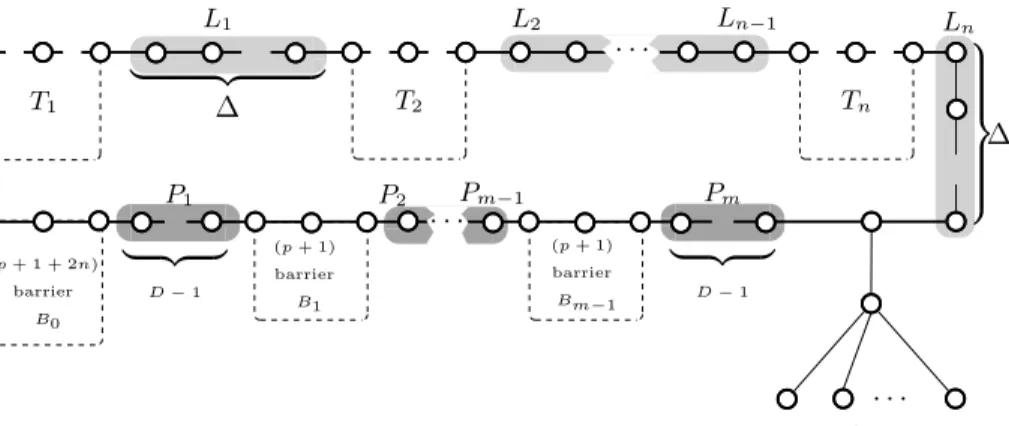
(2) Vol.2010-AL-132 No.6 2010/11/19 IPSJ SIG Technical Report. z. ti }|. .... ... ... | {z } | {z } p−1 p−1. ... | {z } p−1. (a) Ti corresponding to task ti .. |. Monien8) showed the following: Theorem 1. The bandwidth problem is NP-complete for generalized caterpillars of hair length at most 3. We can show the following by a simple modification of the proof of Theorem 1: Theorem 2. The bandwidth problem is NP-complete for convex trees.. { |. ... {z } 2p − 2. Proof. (Sketch.)As in the proof of Theorem 1, we reduce the multiple processor scheduling problem, which is known to be strongly NP-complete, to our problem. Given a set T = {t1 , t2 , . . . , tn } of tasks (ti being the execution time of task i), a deadline D, and the size m of a set {1, 2, . . . , m} of processors, the multiple processor schedule problem asks whether the tasks in T can be scheduled on the m processors satisfying the deadline D. Corresponding to an instance of this problem, a convex tree C is constructed as follows. Each task ti is represented by a caterpillar Ti shown in Figure 1(a). Each processor i is represented by a chain Pi of length D − 1. Special components called “barrier” and “turning point” are constructed as shown in Figure 1(b) and Figure 1(c), respectively. C is constructed from these components as shown in Figure 2. Task caterpillars Ti and Ti+1 are separated by a chain Li of length ∆. Processor chains Pi and Pi+1 are separated by a (p + 1)-barrier Bi . A turning point of height p+2n+1 separates the upper task portion and the lower processor. (b) p-barrier.. ... {z } 2p − 1. (c) Turning point of height p. Fig. 1. Components of caterpillar C.. L1. |. | {z }. barrier. D−1. B0. Ln. T2. Tn. ∆. P2. Pm−1. Pm. .... {. 2.1 NP-completeness Result A caterpillar is a tree in which all the vertices of degree greater than one are contained in a single path called a body. An edge incident to a vertex of degree one is called a hair. A generalized caterpillar is a tree obtained from a caterpillar by replacing each hair by a path. A path replacing a hair is also called a hair.. (p + 1 + 2n). Ln−1. }. P1. 2. Bandwidth of Convex Bipartite Graphs. .... }|. {z ∆. T1. L2. z. therefore for chordal bipartite graphs). Constant-factor polynomial-time approximation algorithms are known for few special graph classes such as AT-free graphs and its subclasses as shown by Kloks, Kratsch, and M¨ uller7) . Convex graphs or 2-directional orthogonal ray graphs are not contained in any of these classes. We provide in Section 2.2 a linear-time 4-approximation algorithm and an O(n log n)time 2-approximation algorithm for convex bipartite graphs, and in Section 3 an O(n2 log n)-time 3-approximation algorithm for 2-directional orthogonal ray graphs, where n is the number of vertices of a graph.. (p + 1). (p + 1). barrier. barrier. B1. Bm−1. | {z } D−1. ... turning point of height p + 1 + 2n. Fig. 2. 2. Instance of bandwidth reduced from multiprocessor scheduling problem. c 2010 Information Processing Society of Japan.
(3) Vol.2010-AL-132 No.6 2010/11/19 IPSJ SIG Technical Report. Let G be a convex bipartite graph with bipartition (X, Y ) and an ordering ≺ of X satisfying the adjacency property with X = {x1 , x2 , . . . , x|X| } and x1 ≺ . . . ≺ x|X| . Assume Y = {1, 2, . . . , |Y |}. Define mappings s : Y → {1, 2, . . . , n} and l : Y → {1, 2, . . . , n} such that for y ∈ Y , xs(y) and xl(y) are, respectively, the smallest and largest vertices in ≺ adjacenct to y. For each vertex y ∈ Y , let m(y) = ⌈(s(y) + l(y))/2⌉. 2.2.1 Algorithm 1 Our first algorithm is described in Figure 3. Algorithm 1 takes as input G along with the mappings s and l and outputs a linear layout π of G. The idea of the algorithm is to lay out the vertices of X in the same order as they appear in ≺ and insert the vertices of y between them, such that for each y ∈ Y , ⌊|N (y)|/2⌋ vertices of the set N (y) of its neighbors are onto its left and the remaining to its right. Algorithm 1 starts by computing m(y) for each vertex of Y and sorting the vertices according to their m(i) values (Lines 1 and 2). It incrementally assigns labels to the vertices of X in the order in which they appear in ≺ ; stopping at each xj to check whether there is a vertex in y with m(y) value equal to j, in which case it assigns the current label to y. The process is repeated until all vertices have been labelled (Lines 3 through 8).. portion. A (p + 2n + 1)-barrier B0 is attached to the left of P1 . If we remove from C the degree-1 vertices of the turning point, the remaining tree is a caterpillar. It is easy to see that a caterpillar is biconvex, and therefore both partitions of C have an ordering satisfying the adjacency property. If we restore the degree-1 vertices, irrespective of their position in the ordering of their partition, they do not disturb the adjacency property of the ordering of the other partition. Thus C is a convex tree. If we set the values of ∆ and p such that ∆ = 2 × (m(D + 2) − 2) and p > 2n(D + 4), it can be shown that the tasks in T can be scheduled on the m processors if and only if C has a bandwidth of k = p + 1 + 2n. In fact, this proof is exactly the same as the proof of Theorem 1, except only for a slight difference in the structure of the turning point. Therefore, we shall only briefly describe the idea of the proof here. For a detailed treatment, we refer to Monien8) . If there exists a scheduling of the tasks in T such that tasks ti1 , ti2 , . . . , tij are assigned to processor i, then C has bandwidth k and an optimal layout can be achieved by (a) laying out the vertices of the body of Ti1 , Ti2 , . . . , Tij between barriers Bi−1 and Bi (betwen Bm−1 and turning point, for i = m) and (b) laying out the vertices of B0 at the extreme left and those of the turning point at the extreme right. Conversely, if C has bandwidth k, then in any optimal layout of C, (a) the turning point must be laid out at one of the extreme ends, and barrier B0 must be laid out at the other, (b) all the vertices of the body of each Tj must be laid out between two barriers Bi and Bi+1 for some i (or Bm−1 and the turning point for i = m − 1), and (c) for each i, if between Bi and Bi+1 (or between Bm−1 and turning point for i = m−1), bodies of Ti1 , Ti2 , . . . , Tij are laid out, then ti1 +ti2 +· · ·+tij < D. This gives us a scheduling of the tasks in T .. 1 2. 3 4 5 6 7 8 9. 2.2 Approximation Algorithms for Convex Bipartite Graphs In this section, we present two algorithms that approximate the bandwidth of convex graphs with worst-case performance ratios of 2 and 4.. Compute m(i) for each vertex i ∈ Y . Add a dummy vertex |Y | + 1 to Y with m(|Y | + 1) = |X| + 1. Let σ(1), . . . , σ(|Y + 1|) be the vertices of Y sorted in the nondecreasing order of m(i) value, where σ is a permutation on {1, . . . , |Y | + 1}. Initialize i ← 1, j ← 1, k ← 1. while (j ≤ |X|) if j < m(σ(i)) π(xj ) = k; j ← j + 1; k ← k + 1. else if j = m(σ(i)) π(σ(i)) = k; i ← i + 1; k ← k + 1. return π Fig. 3. 3. Algorithm 1.. c 2010 Information Processing Society of Japan.
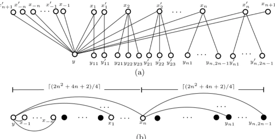
(4) Vol.2010-AL-132 No.6 2010/11/19 IPSJ SIG Technical Report. Consider a layout π output by Algorithm 1. For a vertex y ∈ Y , let Gy be the subgraph of G induced by the vertices in Vy = {v|π(xs(y) ) ≤ π(v) ≤ π(y)} ∪ {v|π(y) ≤ π(v) ≤ π(xl(y) )}. The diameter of a graph is the least integer k such that a shortest path between any pair of vertices of the graph is at most k. Lemma 3. The diameter of Gy is at most 4.. ⌈(|Vy | − 1)/4⌉. Thus we have: |Vy′ | − 1 bπ (G) ≤ b(G) (|Vy | − 1)/4 Since the order of X in ≺ is preserved in π, x must be xs(y) or xl(y) , and therefore Vy′ ⊆ Vy . Thus we get: bπ (G) ≤ 4. b(G). Proof. Let u, v be a pair of vertices of Vy . Consider first the case that both u, v ∈ Vy ∩ X. Since π preserves the ordering ≺ of X, u must be xi and v must be xj for some s(y) ≤ i, j ≤ l(y). Thus both u and v are adjacent to y. Hence the distance between u and v is 2. Consider next the case that u ∈ Vy ∩ X and v ∈ Vy ∩ Y . Vertex v must be adjacent to at least one vertex u′ in Vy ∩ X. If not, then it must be that v is connected to some xj with j < s(y) or j > l(y), which means that m(v) < s(y) or m(v) > l(y), contradicting the assumption that Algorithm 1 placed v between xs(y) and y or between x(l(y) and y. If u = u′ , then the distance between u and v is 2. Else, both u and u′ are at distance 2 from the earlier case, and therefore u and v are at a distance 3. Consider finally the case that both u, v ∈ Vy ∩ Y . From the earlier case u must be adjacent to some vertex u′ , v must be adjacent to some vertex v ′ . Also u′ and v ′ are both adjacent to y. Hence the distance between u and v is at most 4. In all the above cases, the shortest path between any pair of vertices does not exceed 4, and thus we have the lemma.. There exist graphs for which this ratio is asymptotically equal to 4. Figure 4(a) shows an example of such a graph. Let us assume that the mappings s and l provided to Algorithm 1 are based on the left to right ordering of the vertices of the upper partition as shown in Figure 4(a). The layout π returned by Algorithm 1 will lay out between y and xn+1 all the vertices ′ xi , x′i , yij , yij (1 ≤ i ≤ n, 1 ≤ j ≤ 2n − 1). Thus bπ (G) = 2n2 + 2n + 1. On the other hand, the diameter of this graph is 4, and so from Lemma 4, x′n+1 x′−n x−n. x′. . . .−1. x−1. ′ x1 x1. x′2. x2. .... ... ′ ′ ′ ′ y22 y23 y11 y11 y21 y22 y23 y21. y. yn1. xn+1. x′n. xn. .... ′ yn,2n−1 yn1. ′ yn,2n−1. (a). The following is a well-known lower bound for the bandwidth of a graph1) . Lemma 4. For a graph G, b(G) ≥ max⌈(N ′ − 1)/D′ ⌉, where the maximum is taken over all connected subgraphs G′ of G, N ′ is the number of vertices of G′ , and D′ is the diameter of G′ . We are now ready to show the approximation ratio of Algorithm 1. Lemma 5. For layout π returned by Algorithm 1, bπ (G) ≤ 4 × b(G).. 2. ⌈(2n2 + 4n + 2)/4⌉. ⌈(2n + 4n + 2)/4⌉. .... ... y x−1. . . .x. ... −n. x1. .... xn. .... ... yn1. yn,2n−1. (b) Fig. 4. Proof. Let (x, y), x ∈ X, y ∈ Y be an edge of G such that |π(x) − π(y)| = bπ (G). Let Vy′ be the set of vertices v such that v lies between x and y in π. Then bπ (G) = |Vy′ | − 1. On the other hand, from Lemmas 3 and 4, we get b(G) ≥. 4. (a)An example for which the approximation ratio of Algorithm 1 is asymptotically equal to 4. (b) A layout with bandwidth ⌈(2n2 + 4n + 2)/4⌉. Only the half right of y is shown as the left half contains the primed counterparts in a symmetric layout. The regions denoted by black vertices denote the vertices yij , which can be laid out within the same bandwidth.. c 2010 Information Processing Society of Japan.
(5) Vol.2010-AL-132 No.6 2010/11/19 IPSJ SIG Technical Report. b(G) ≥ ⌈(2n2 + 4n + 2)/4⌉. In fact, for large values of n, there is a layout of bandwidth ⌈(2n2 + 4n + 2)/4⌉, as shown in Figure 4(b). Thus the approximation ratio bπ (G)/b(G) is aymptotically equal to 4. Algorithm 1 can be implemented to run in O(|X| + |Y |) time. So it follows from Lemma 5 that: Theorem 6. Algorithm 1 computes a linear layout of a convex graph G with bipartition (X, Y ) in O(|X| + |Y |) time such that bπ (G) ≤ 4 × b(G). If only G, and not s and l, is given, we can compute an ordering satisfying the adjacency property (and thus s and l) in time linear to the number of vertices and edges of the graph, as shown by Booth and Lueker3) . In that case, the time complexity would be O(|X| + |Y | + |E|), where E is the edge set of G. In the next subsection, we show a different algorithm that runs slower but improves the approximation ratio to 2. 2.2.2 Algorithm 2 Let G be a convex bipartite graph with bipartition (X, Y ) and an ordering ≺ of X satisfying the adjacency property with X = {x1 , x2 , . . . , x|X| } and x1 ≺ . . . ≺ x|X| . Let s and l be mappings defined in Section 2.2.1. Let GI be a graph obtained from G by adding to it an edge (y1 , y2 ) for each pair y1 ,y2 ∈ Y having a common neighbor. A graph is said to be an interval graph if for every vertex of the graph, there exists an interval on the real line, such that two intervals intersect if and only if their corresponding vertices are adjacent. Lemma 7. GI is an interval graph.. Lemma 9. For an interval graph with n vertices, the bandwidth problem can be solved in O(n log n) time if the interval model is provided. Given a convex bipartite graph G and mappings s and l, Algorithm 2 simply constructs the interval model of GI and applies the algorithm for interval graphs. The interval model of GI can be constructed from s and l in time linear to the number of vertices in G, and therefore we have from Lemmas 8 and 9 the following theorem: Theorem 10. Algorithm 2 computes a linear layout π of a convex graph G with n vertices in O(n log n) time such that bπ (G) ≤ 2 × b(G). For a path of length 3, whose bandwidth is 1, Algorithm 2 may return a layout of bandwidth 2. Therefore the above-mentioned bound is tight. 3. Bandwidth of 2-directional Orthogonal Ray Graphs Since the set of convex bipartite graphs is a proper subset of the set of twodirectional orthogonal ray graphs, the bandwidth problem is NP-complete for 2-directional orthogonal ray graphs, by Theorem 2. In this section, we show a 3-approximation algorithm for 2-directional orthogonal ray graphs. Let G be a bipartite graph with bipartition (X, Y ), and let (≺X , ≺Y ) be a pair of orderings of X and Y , respectively. Two edges (x, y) and (x′ , y ′ ) of G are said to cross in (≺X , ≺Y ) if x′ ≺X x and y≺Y y ′ . If for every pair (x, y) and (x′ , y ′ ) that cross, (x′ , y) is also an edge of G, then (≺X , ≺Y ) is said to be a weak ordering of G. If for every pair (x, y) and (x′ , y ′ ) of crossing edges, both (x, y ′ ) and (x′ , y) are edges of G, then (≺X , ≺Y ) is said to be a strong ordering of G. Spinrad, Brandst¨adt, and Stewart11) gave the following characterization of bipartite permutation graphs. Lemma 11. A graph G is a bipartite permutation graph if and only if G has a strong ordering. In an earlier work10) , we showed the following characterization of 2-directional orthogonal ray graphs. Lemma 12. A graph G is a 2-directional orthogonal ray graph if and only if G has a weak ordering. Given a 2-directional orthogonal ray graph G with bipartition (X, Y ), edge set E, and a weak ordering (≺X , ≺Y ) of G, we can construct a graph GBP having. Proof. We can see that GI is an interval graph by defining interval [i, i] for each vertex xi ∈ X , and interval [s(y), l(y)] for each vertex y ∈ Y . Lemma 8. b(GI ) ≤ 2b(G) Proof. Let π be an optimal layout of G. Consider the bandwidth of the same layout of graph GI . For edge (u, v) ∈ E(G) ∩ E(GI ), π(u) − π(v) ≤ b(G). For edge (u, v) ∈ E(GI ) \ E(G), there exists a common neighbor of u and v in G, and therefore π(u) − π(v) ≤ 2b(G). Thus bπ (GI ) ≤ 2b(G). Since b(GI ) ≤ bπ (GI ), we get b(GI ) ≤ 2bπ (G). Sprague12) showed the following about interval graphs.. 5. c 2010 Information Processing Society of Japan.
(6) Vol.2010-AL-132 No.6 2010/11/19 IPSJ SIG Technical Report. order of y2′ and y1 in ≺Y . Case 3.3.1. y2′ = y1 : since (x2 , y1 ) = (x2 , y2′ ), we have (x2 , y1 ) ∈ E ⊆ EBP Case 3.3.2. y2′ ≺Y y1 : since (x2 , y2′ ) ∈ E and (x′1 , y1 ) ∈ E cross, (x2 , y1 ) ∈ E ′ ⊆ EBP . Case 3.3.3. y1 ≺Y y2′ : since (x1 , y1 ) ∈ E ′ \ E and (x2 , y2′ ) ∈ E cross, we have (x2 , y1 ) ∈ EBP from Case 2. In all the above subcases of Case 3, we have shown that (x1 , y1 ) ∈ EBP , and hence both (x2 , y1 ), (x1 , y2 ) ∈ EBP . Thus we have shown that for every e1 = (x1 , y1 ) and e2 = (x2 , y2 ) of GBP that cross in (≺X , ≺Y ), both (x2 , y1 ) and (x1 , y2 ) are also edges of GBP ; and therefore from Lemma 11, GBP is a bipartite permutation graph.. vertex set VBP = X ∪Y and edge set EBP = E ∪E ′ , where E ′ is the set consisting of an edge (x, y ′ ) for every pair of edges (x, y) and (x′ , y ′ ) that cross in (≺X , ≺Y ). Lemma 13. GBP is a bipartite permutation graph. Proof. We will show that GBP is a bipartite permutation graph by showing that (≺X , ≺Y ) is a strong ordering of GBP . Let e1 = (x1 , y1 ) and e2 = (x2 , y2 ) be two edges of GBP that cross in (≺X , ≺Y ). We distinguish three cases: Case 1. both e1 , e2 ∈ E, Case 2. one each of e1 , e2 is in E ′ \ E and E, and Case 3. both e1 , e2 ∈ E ′ \ E. Case 1: Since (≺X , ≺Y ) is a weak ordering of G, (x2 , y1 ) ∈ E. By definition of E ′ , (x1 , y2 ) ∈ E ′ . Hence both (x2 , y1 ), (x1 , y2 ) ∈ EBP . Case 2: Without loss of generality, assume e1 ∈ E ′ \ E and e2 ∈ E. By definition of E ′ , e1 ∈ E ′ \ E implies that there exist y1′ ≺Y y1 and x′1 ≺X x1 such that (x1 , y1′ ), (x′1 , y1 ) ∈ E and they cross. Since (x1 , y1′ ) and (x2 , y2 ) also cross, (x1 , y2 ) must be in E ′ and therefore in EBP . To see that (x2 , y1 ) ∈ EBP , we further distinguish three cases depending on the order of x′1 and x2 in ≺X . Case 2.1. x′1 = x2 : (x2 , y1 ) = (x′1 , y1 ) and hence (x2 , y1 ) ∈ E ⊆ EBP . Case 2.2. x2 ≺X x′1 : since (x′1 , y1 ) and (x2 , y2 ) cross, (x2 , y1 ) ∈ E ⊆ EBP . Case 2.3. x′1 ≺X x2 : since (x1 , y1′ ) and (x2 , y2 ) cross, (x2 , y1′ ) ∈ E; Moreover, (x2 , y1′ ) and (x′1 , y1 ) cross, implying that (x2 , y1 ) ∈ E ′ ⊆ EBP . In all the above subcases of Case 2, we have shown that (x2 , y1 ) ∈ EBP , and hence both (x2 , y1 ), (x1 , y2 ) ∈ EBP . Case 3: By definition of E ′ , e1 ∈ E ′ \ E implies that there exist y1′ ≺Y y1 and x′1 ≺X x1 such that (x1 , y1′ ), (x′1 , y1 ) ∈ E and they cross. Again by definition of E ′ , e2 ∈ E ′ \ E implies that there exist y2′ ≺Y y2 and x′2 ≺X x2 such that (x2 , y2′ ),(x′2 , y2 ) ∈ E and they cross. Since (x1 , y1′ ) and (x′2 , y2 ) also cross, (x1 , y2 ) must be in E ′ and therefore in EBP . To see that (x2 , y1 ) ∈ EBP , we further distinguish three cases depending on the order of x′1 and x2 in ≺X . Case 3.1. x′1 = x2 : since (x2 , y1 ) = (x′1 , y1 ), we have (x2 , y1 ) ∈ E ⊆ EBP . Case 3.2. x2 ≺X x′1 : since (x′1 , y1 ) ∈ E and (x2 , y2 ) ∈ E ′ \E cross, we have (x2 , y1 ) ∈ EBP from Case 2. Case 3.3. x′1 ≺X x2 : we further distinguish three cases, depending on the. Lemma 14. b(GBP ) ≤ 3 × b(G). Proof. Let π be an optimal layout of G. Consider the same layout of GBP . For an edge (x, y) of G ∩ GBP , |π(x) − π(y)| ≤ b(G). For an edge (x, y) of GBP \ G, there exist vertices x′ ∈ X and y ′ ∈ Y such that (y, x′ ), (x′ , y), (y ′ , x) are edges of G, and therefore |π(x) − π(y)| ≤ 3 × b(G) . Thus we have bπ (GBP ) ≤ 3b(G). Since b(GBP ) ≤ bπ (GBP ), we get b(GBP ) ≤ 3 × b(G). We shall assume that along with a 2-directional orthogonal ray graph G, a weak ordering (≺X , ≺Y ) is also provided as input. If not, then such an ordering as be computed in O(n2 ) time, where n is the number of vertices of G10) . We can construct GBP from G in O(n2 ) time. This can be done by first remembering for each x ∈ X, its smallest neighbor yx in ≺Y and for each y ∈ Y , its smallest neighbor xy in ≺X , and then adding to G an edge (x, y) for each pair x, y for which yx ≺ y and xy ≺ x. Uehara13) showed that an optimal layout of a n-vertex bipartite permutation graph having bandwidth k can be computed in O(n2 log k) time. Then it follows from Lemma 14 that: Theorem 15. There is an O(n2 log n)-time algorithm which computes a linear layout π of an n-vertex 2-directional orthogonal ray graph G such that bπ (G) ≤ 3 × b(G).. 6. c 2010 Information Processing Society of Japan.
(7) Vol.2010-AL-132 No.6 2010/11/19 IPSJ SIG Technical Report. 5) Heggernes, P., Kratsch, D. and Meister, D.: Bandwidth of bipartite permutation graphs in polynomial time, J. of Discrete Algorithms, Vol. 7, No. 4, pp. 533–544 (2009). 6) Kloks, T., Kratsch, D. and Mu¨ uller, H.: Bandwidth of chain graphs, Inf. Process. Lett., Vol.68, No.6, pp.313–315 (1998). 7) Kloks, T., Kratsch, D. and Mu¨ uller, H.: Approximating the Bandwidth for Asteroidal Triple-Free Graphs, Journal of Algorithms, Vol.32, pp.41–57 (1999). 8) Monien, B.: The bandwidth minimization problem for caterpillars with hair length 3 is NP-complete, SIAM J. Algebraic Discrete Methods, Vol.7, No.4, pp.505–512 (1986). 9) Papadimitriou, C.: The NP-Completeness of the bandwidth minimization problem, Computing, Vol.16, pp.263–270 (1976). 10) Shrestha, A. M.S., Tayu, S. and Ueno, S.: On Orthogonal Ray Graphs, Discrete Applied Mathematics, Vol.158, pp.1650–1659 (2010). 11) Spinrad, J., Brandst¨ adt, A. and Stewart, L.: Bipartite permutation graphs, Discrete Appl. Math., Vol.18, No.3, pp.279–292 (1987). 12) Sprague, A.P.: An O(n log n) algorithm for bandwidth of interval graphs, SIAM J. Discrete Math, Vol.7(2), pp.213–220 (1994). 13) Uehara, R.: Bandwidth of bipartite permutation graphs, 19th Annual International Symposium on Algorithms and Computation, Lecture Notes in Computer Science, Vol.5369, pp.824–835 (2008). 14) Unger, W.: The Complexity of the Approximation of the Bandwidth Problem, FOCS ’98: Proceedings of the 39th Annual Symposium on Foundations of Computer Science, pp.82–91 (1998).. 4. Bandwidth of Biconvex Trees The 2-claw is a graph obtained from the complete bipartite graph K13 by replacing each edge by a path of length 2. The following lemma can be quickly verified. Lemma 16. The 2-claw is not a biconvex tree. Biconvex trees can be characterized as follows: Lemma 17. A tree T is biconvex if and only if T is a caterpillar. Proof. The sufficiency is easy. To prove the necessity, suppose T is a biconvex graph. Let P be a longest path in T . If the length of P is less than five, T is trivially a caterpillar, and so we assume that it is greater than five. Suppose there exists a vertex not in P having degree greater than 1. This implies that T contains the 2-claw as a subtree, contradicting the assumption that T is biconvex graph. Therefore T is a caterpillar. Assmann, Peck, Syslo, and Zak showed the following: Lemma 18. The bandwidth of generalized caterpillars of hair length at most two can be computed in linear time. From Lemma 17 and Lemma 18, we have: Theorem 19. The bandwidth of biconvex trees can be computed in linear time. We conclude this paper with a note that the complexity of bandwidth problem for biconvex graphs is open. References 1) Assmann, S.F., Peck, G.W., Syslo, M.M. and Zak, J.: The Bandwidth of Caterpillars with Hairs of Length 1 and 2, SIAM Journal on Algebraic and Discrete Methods, Vol.2, No.4, pp.387–393 (1981). 2) Blache, G., Karpinski, M. and Wirtgen, J.: On Approximation Intractability of the Bandwidth Problem, Technical report, University of Bonn (1997). 3) Booth, K.S. and Lueker, G.S.: Testing for the consecutive ones property, interval graphs, and graph planarity using PQ-tree algorithms, Journal of Computer and System Sciences, Vol.13, No.3, pp.335 – 379 (1976). 4) Brandst¨ adt, A., Le, V.B. and Spinrad, J.P.: Graph classes: a survey, Society for Industrial and Applied Mathematics (1999).. 7. c 2010 Information Processing Society of Japan.
(8)
図
関連したドキュメント
In an n by n complete bipartite graph with independent exponentially distributed edge costs, we ask for the minimum total cost of a set of edges of which each vertex is incident to
Perhaps the most significant result describing planar graphs as intersection graphs of curves is the recent proof of Scheinerman’s conjecture that all planar graphs are segment
The scarcity of Moore bipartite graphs, together with the applications of such large topologies in the design of interconnection networks, prompted us to investigate what happens
It can be shown that cubic graphs with arbitrarily large girth exist (see Theorem 3.2) and so there is a well-defined integer µ 0 (g), the smallest number of vertices for which a
The following variation was considered by Beineke and Schwenk [1] and also by Irving [5]: for 1 ≤ m ≤ n, the bipartite Ramsey number R(m, n) is the smallest integer r such that
Kilbas; Conditions of the existence of a classical solution of a Cauchy type problem for the diffusion equation with the Riemann-Liouville partial derivative, Differential Equations,
Turmetov; On solvability of a boundary value problem for a nonhomogeneous biharmonic equation with a boundary operator of a fractional order, Acta Mathematica Scientia.. Bjorstad;
In this paper, we strengthen this NP-completeness result by showing that the Outer- connected Domination Decision problem remains NP-complete for perfect elimination bipartite
