オプティカルフローと独立成分分析によるドミナントプレーン検出

全文

(1)2005−CVIM−149（1） 2005／5／12. 社団法人情報処理学会研究報告 IPSJ SIG Technical Report. オプティカルフローと独立成分分析によるドミナントプレーン検出大西直哉 †. 井宮淳 ††. †. 千葉大学自然科学研究科千葉大学総合メディア基盤センター〒 263-8522 千葉市稲毛区弥生町 1-33. ††. あらましドミナントプレーンとは画像の最大領域を占める平面であり、それを検出することはロボットナビゲーションなどにおいて有益である。本論文では、移動するカメラから得られるオプティカルフローに対して独立成分分析を行うことで、ドミナントプレーンを検出するアルゴリズムを提案する。障害物が含まれないシーンから得られるオプティカルフローと、障害物が含まれたシーンから得られるオプティカルフローを独立成分分析の入力値として用いる。出力結果に統計的な処理を施し、ドミナントプレーンの領域を検出する。実画像を用いた実験結果を示す。. Dominant plane detection using optical flow and Independent Component Analysis Naoya OHNISHI† and. Atsushi IMIYA††. †School of Science and Technology, Chiba University ††Institute of Media and Information Technology, Chiba University Yayoi-cho 1-33, Inage-ku, 263-8522, Chiba, Japan. Abstract Dominant plane is an area which occupies the largest domain in the image. The dominant plane estimation is an essential task for the autonomous navigation and the path planning of the mobile robot equipped with a vision system, since the robot moves on the dominant plane. In this paper, we develop an algorithm for dominant plane detection using optical flow and Independent Component Analysis. Since the optical flow field is a mixture of flows of the dominant plane and the other area, we separate the dominant plane using Independent Component Analysis. Using the initial data as a supervisor signal, the robot detects the dominant plane. For each image in a sequence, the dominant plane corresponds to an independent component. This relation provides us a statistical definition of the dominant plane. Experimental results using real image sequence show that our method is robust against the non-unique velocity of the mobile robot.. 1. Introduction. In this work, we aim to develop an algorithm for dominant plane detection using the optical flow observed by means of a vision system mounted on a mobile robot. The dominant plane is a planar area which occupies the largest domain in the image observed by a camera. Assuming that the robot moves on the dominant plane (e.g., floors and ground areas), dominant plane estimation is an essential task for the autonomous navigation and the path planning of the mobile robot. For the autonomous navigation of mobile robots, vision sensors and sonar or laser sensors are generally used. Sonar and laser sensors [1] provide simple methods of obstacle detection. These sensors are effective in obstacle detection for collision avoidance, since these methods can obtain range information to an ob-. ject. On the other hand, stationary vision sensors have difficulty in obtaining range information. However, vision sensors mounted on a mobile robot can obtain an image sequence from the camera motion. The image sequence provides the motion and structure from correspondences of points on successive images [2]. Additionally, vision sensors are fundamental devices for the understanding of the environment, since the robot collaborates with a human being. Moreover, visual information is valid for the path planning of the mobile robot in a long sequence, because the vision system can capture environmental information quickly for a large area compared to present sonar- and laser-based systems. There are many methods for the detection of obstacles or planar areas using vision systems [3]. For example, the edge detection of omni and monocular. 1 −1−.

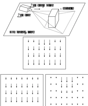
(2) camera systems [4] and the observation of landmarks [5] are the classical ones. However, since these methods are dependent on the environment around a robot, they are difficult to apply in general environments. If a robot captures an image sequence of moving objects, the optical flow [6] [7] [8], which is the motion of the scene, is obtained for the fundamental features in order to construct environment information around the mobile robot. Additionally, the optical flow is considered as fundamental information for the obstacle detection in the context of biological data processing [9]. Therefore, the use of optical flow is an appropriate method from the viewpoint of the affinity between the robot and human being. The obstacle detection using optical flow is proposed in [10] [11]. Enkelmann [10] proposed an obstacle-detection method using the model vectors from motion parameters. Santos-Victor and Sandini [11] also proposed an obstacle-detection algorithm for a mobile robot using the inverse projection of optical flow to ground floor, assuming that the motion of the camera system mounted on a robot is pure translation with a uniform velocity. However, even if a camera is mounted on a wheel-driven robot, the vision system does not move with uniform velocity due to mechanical errors of the robot and unevenness of the floor. Independent Component Analysis(ICA) [12] provides a powerful method for texture analysis, since ICA extracts dominant features from textures as independent components [13][14]. Optical flow is a texture yielded on surfaces of objects in an environment observed by a moving camera. Therefore, it is possible to extract independent features form flow vectors on pixels dealing with flow vectors as textons. Consequently, we use ICA to separate the dominant plane and the other area. In Section 2, we briefly present ICA, and we show that separation of pixels in a scene applies ICA to flow vectors of pixels. Section 3 presents an algorithm for the detection of the dominant plane from optical flow. In Section 4, we show experiments for the detection of the dominant plane using a real image sequence observed by the camera mounted on a mobile robot. we show the validity of own method for a robot navigation.. 2. Application of ICA to optical flow. ICA [12] is a statistical technique for the separation of original signals from mixture signals. Assume that the mixture signals x1 (t) and x2 (t) are expressed as a linear combination of the original signals s1 (t) and s2 (t), that is, x1 (t) = a11 s1 (t) + a12 s2 (t),. x2 (t) = a21 s1 (t) + a22 s2 (t),. (2). where a11 , a12 , a21 , and a22 are weight parameters of the linear combination. Using only the recorded signals x1 (t) and x2 (t) as an input, ICA can estimate the original signals s1 (t) and s2 (t) based on the statistical properties of these signals. We apply ICA to the optical flow observed by a camera mounted on a mobile robot for detection of the feasible region on which the robot can move. The optical-flow fields are suitable for the input signals to ICA, since the optical flow observed by the moving camera is expressed as the linear combination of the motion field of the dominant plane and the other objects, as shown in Fig1. Assuming that the motion field of the dominant plane and the other objects are spatially independent components, ICA enables us to detect the dominant plane on which robot can moves. For each image in a sequence, we assume that optical flow vectors in the dominant plane corresponds to an independent component. as shown in Fig.2.. Camera Motion Obstacle Camera. Dominant Plane. Figure 1: Top-left: Example of camera displacement and the environment with obstacles. Top-right: Optical flow observed through the moving camera. Bottom-left: The motion field of the dominant plane. Bottom-right: The motion field of the other objects. The optical flow(top-right) is expressed as the linear combination of bottom motion fields.. (1) 2 −2−.

(3) 3.1. y. ˆ y, t) at time t First, we capture image sequence I(x, without obstacles as shown in Fig.4 and compute opdy tical flow u(t) ˆ = ( dx dt , dt ) as. u(t0) u(t1). t0. t1. u(t2). t2. Learning supervisor signal. t3 u(t3) t4. t5 u(t4). x. ˆ y, t) + Iˆt = 0, ˆ > ∇I(x, u(t). t u(t5). (3). where x and y are the pixel coordinates of a image. For the detail of the computation of this equation, see [6][7][8].. Figure 2: Dominant vector detection in a sequence of images. u(ti ) corresponds to the dominant vector which defines the dominant plane at time ti .. Camera motion Camera. 3. Algorithm for dominant plane detection from image sequence. Dominant Plane. In this section, we develop an algorithm for the detection of the dominant plane from the image sequence observed by a camera mounted on a mobile robot. When the camera mounted on the mobile robot moves on the ground plane, we obtain successive images which include a dominant plane area and obstacles. Assuming that the camera is mounted on a mobile robot, the camera moves parallel to the dominant plane. Since the computed optical flow from the successive images describes the motion of the dominant plane and obstacles on the basis of the camera displacement, the difference between these optical flow vectors enables us to detect the dominant plane area. The difference of the optical flow is shown in Fig.3. Camera displacement T Image Plane Camera. Optical flow. Figure 4: Captured image sequence without obstacles. Top: Example of camera displacement and the environment without obstacles. Bottom-left: An image ˆ y, t). Bottom-right: Comof the dominant plane I(x, puted optical flow u(t). ˆ. Obstacle. T. Dominant plane. After we compute the optical flow u(t), ˆ frame t = 0 . . . n, we create the supervisor signal u, ˆ. T. Figure 3: The difference of the optical flow between the dominant plane and obstacles. If the camera moves in the distance T parallel to the dominant plane, optical flow vector at the obstacles area in the image plane shows that the obstacle moves in the distance T , or optical flow vector at the dominant plane area in the image plane shows that the dominant plane moves in the distance T . Therefore, the camera observes difference optical flow vector between the dominant plane and obstacles.. n. ˆ= u. 3.2. 1X ˆ u(t). n t=0. (4). Dominant plane detection using ICA. Next, we capture image sequence I(x, y, t) with obstacles as shown in Fig.5 and compute optical flow u(t) in the same way. The optical flow u(t) and the supervisor signal u ˆ are used as an input signal for ICA. Setting v1 and v2 to. 3 −3−.

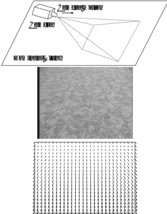
(4) Since the dominant plane occupies the largest domain in the image, we compute the distance between l and the median of l. Setting m to be the median value of the elements in the vector l, the distance d = (d(1), d(2), . . . , d(xy))> is. Camera Motion Obstacle Camera. d(i) = |l(i) − m|.. Dominant Plane. (7). We detect the area on which d(i) ≈ 0, as the dominant plane.. 3.3. Procedure for dominant plane detection. Our algorithm is summarized as follows. phase is,. Learning. 1. Robot moves on the dominant plane in the small distance. ˆ v, t) of dominant 2. Robot captures a image I(u, plane. 3. Compute the optical flow u(t) ˆ between the images ˆ v, t) and I(u, ˆ v, t − 1). I(u,. Figure 5: Optical flow of the image sequence. Top: Example of camera displacement and the environment with obstacles. Bottom-left: An image of the dominant plane and obstacles I(x, y, t). Bottom-right: Computed optical flow u(t). In a top-middle area, where exists the obstacle, the lengths of optical flow vectors are longer than the flow vectors in the other area. be the output signals of ICA, v1 and v2 are ambiguity of the order of the each components. We solve this problem using the difference between the variance of the length of v1 and v2 . Setting l1 and l2 to be the length of v1 and v2 , q 2 + v 2 , (j = 1, 2) (5) lj = vxj yj where vxj and vyj are arrays of x and y axis components of output vj , respectively, the variance σj2 are σj2 =. 1 X 1 X (lj (i) − ¯lj )2 , ¯lj = lj (i), xy i∈xy xy i∈xy. (6). where lj (i) is the ith data of the array lj . Since the motions of the dominant plane and obstacles in the image is different, the output which expresses the obstacle-motion has larger variance than the output which expresses the dominant plane motion. Therefore, if σ12 > σ22 , we detect dominant plane using output signal l as l = l1 , else we use output signal l = l2 .. 4. If time t > n, compute the supervisor signal u ˆ using Eq.(4). Else go to step 1. Next, dominant plane recognition phase is, 1. Robot moves in the environment with obstacles in the small distance. 2. Robot captures a image I(u, v, t). 3. Compute the optical flow u(t) between the images I(u, v, t) and I(u, v, t − 1). 4. Input the optical flow u(t) and the supervisor signal u ˆ to ICA, and output the signal v1 and v2 . 5. Detect the dominant plane using the algorithm Section 3.2. Figure 6 shows the procedure for dominant plane detection using optical flow and ICA.. 4. Experiment. We show experiment for the dominant plane detection using the procedure in Section 3. First, the robot equipped with a single camera moves forward with uniform velocity on the dominant plane and capture the image sequence without obstacles until n = 20. For the computation of optical flow, we use the Lucas-Kanade method with pyramids [15]. Using Eq.(4), we compute the supervisor signal u. ˆ Figure 7 shows the captured image and the computed supervisor signal u. ˆ. 4 −4−.

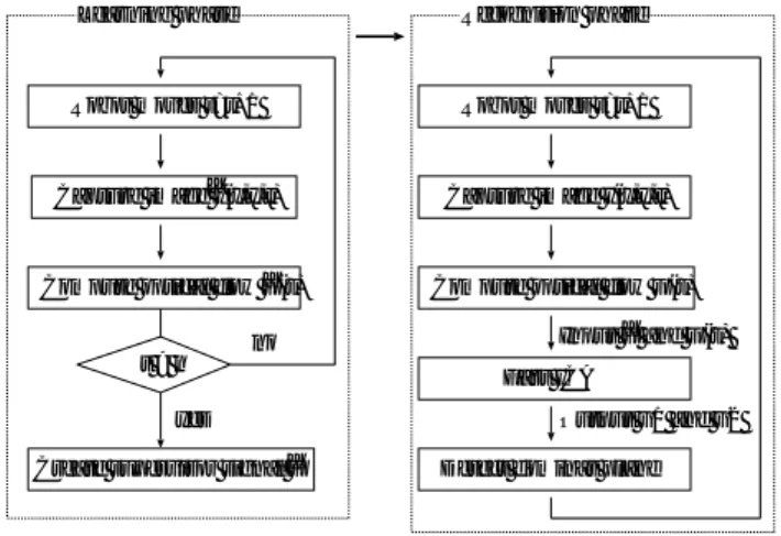
(5) Learning phase. Recognition phase. Robot moves t=t+1. Robot moves t=t+1. Capture image^I(x,y,t). Capture image I(x,y,t). ^ Compute optical flow u(t). Compute optical flow u(t). no t>n yes Create supervisor signal ^ u. ^ and u(t) Input u Fast ICA Output v1 and v2 Detect dominat plane. Figure 6: Procedure for dominant plane detection using optical flow and ICA.. Next, the mobile robot moves on the dominant plane toward the obstacle, as shown in Fig.8. The captured image sequence and computed optical flow u(t) is shown in the first and second rows in Fig.9, respectively. The optical flow u(t) and supervisor signal ˆ are used as an input signal for fast ICA. We use the u Fast ICA package for MATLAB [16] for the computation of ICA. The result of ICA is shown in the third row in Fig.9.. 5. ˆ y, t) of the domiFigure 7: Left: Image sequence I(x, nant plane. Right: Optical flow u ˆ used for the supervisor signal.. Conclusion. We developed an algorithm for the dominant plane detection from a sequence of images observed through a moving uncalibrated camera. The use of the ICA for the optical flow enables the robot to detect a feasible region in which robot can move without requiring camera calibration. These experimental results support the application of our method to the navigation and path planning of a mobile robot with a vision system. For each image in a sequence, the dominant plane corresponds to an independent component. This relation provides us a statistical definition of the dominant plane. The future work is autonomous robot navigation using our algorithm of dominant plane detection. If we project the dominant plane of the image plane onto the ground plane using a camera configuration, the robot detects the movable region in front of the robot in an environment. Since we can obtain the sequence of the dominant plane from optical flow, the robot can move the dominant plane in a space without collision to obstacles.. Figure 8: Experimental environment. The obstacle exists in front of the mobile robot. The mobile robot moves toward the obstacle.. References [1] Hahnel, D., Triebel, R., Burgard, W., and Thrun, S., Map building with mobile robots in dynamic environments, In Proc. of the IEEE ICRA’03, (2003). [2] Huang, T. S. and Netravali, A. N., Motion and structure from feature correspondences: A review, Proc. of the IEEE, 82, 252-268, (1994). [3] Guilherme, N. D. and Avinash, C. K., Vision for mobile robot navigation: A survey IEEE Trans. on PAMI, 24, 237-267, (2002). [4] Kang, S.B. and Szeliski, R., 3D environment modeling from multiple cylindrical panoramic images, Panoramic Vision: Sensors, Theory, Applications, 329-358, Ryad Benosman and Sing Bing Kang, ed., Springer-Verlag, (2001).. 5 −5−.

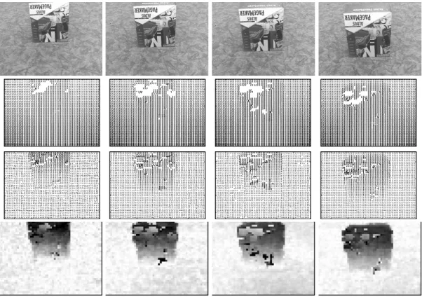
(6) Figure 9: The first, second, third, and forth rows show observed image I(x, y, t), computed optical flow u(t), output signal v(t), and image of the dominant plane D(x, y, t), respectively. In the image of the dominant plane, the white areas are the dominant planes and the black areas are the obstacle areas. Starting from the left column, t = 340, 359, 374, and 393. [5] Fraundorfer, F., A map for mobile robots consisting of a 3D model with augmented salient image features, 26th Workshop of the Austrian Association for Pattern Recognition, 249-256, (2002). [6] Barron, J.L., Fleet, D.J., and Beauchemin, S.S., Performance of optical flow techniques, International Journal of Computer Vision, 12, 43-77, (1994). [7] Horn, B. K. P. and Schunck, B.G., Determining optical flow, Artificial Intelligence, 17, 185-203, (1981). [8] Lucas, B. and Kanade, T., An iterative image registration technique with an application to stereo vision, Proc. of 7th IJCAI, 674-679, (1981). [9] Mallot, H. A., Bulthoff, H. H., Little, J. J., and Bohrer, S., Inverse perspective mapping simplifies optical flow computation and obstacle detection, Biological Cybernetics, 64, 177-185, (1991).. [12] Hyvarinen, A. and Oja, E., Independent component analysis: algorithms and application, Neural Networks, 13, 411-430, (2000). [13] van Hateren, J., and van der Schaaf, A., Independent component filters of natural images compared with simple cells in primary visual cortex, Proc. of the Royal Society of London, Series B, 265, 359-366, (1998). [14] Hyvarinen, A. and Hoyer, P., Topographic independent component analysis, Neural Computation, 13, 1525-1558, (2001). [15] Bouguet, J.-Y., Pyramidal implementation of the Lucas Kanade feature tracker description of the algorithm, Intel Corporation, Microprocessor Research Labs, OpenCV Documents, (1999). [16] Hurri, J., Gavert, H., Sarela, J., and Hyvarinen, A., The FastICA package for MATLAB, website: http://www.cis.hut.fi/projects/ica/fastica/. [10] Enkelmann, W., Obstacle detection by evaluation of optical flow fields from image sequences, Image and Vision Computing, 9, 160-168, (1991). [11] Santos-Victor, J. and Sandini, G., Uncalibrated obstacle detection using normal flow, Machine Vision and Applications, 9, 130-137, (1996). 6 −6−.

(7)