Levenshteinオートマトンのトライへの拡張を元にした近似文字列マッチング

Levenshtein

オートマトンのトライへの拡張を元にした

近似文字列マッチング

Approximate String Matching Based on

Extending Levenshtein Automata for Tries

宮近 充裕

_{吉仲 亮}

_{山本 章博}

Atsuhiro Miyachika

_{Ryo Yoshinaka}

_{Akihiro Yamamoto}

1

_{京都大学 情報学研究科}

1

_{Graduate School of Informatics, Kyoto University}

Abstract: In this paper, we treat an approximate string matching problem: to enumerate all strings stored in a given set of strings, called a dictionary, whose edit distance from a given query string does not exceed a given threshold. Approximate string matching is used in various fields such as text retrieval and finding similar DNA subsequences in computational biology. We give some methods for solving the approximate string matching problem, by extending Levenshtein automaton, which is known as a method for finding all occurrences of words which approximately match a query word in a long text. We further design a DFA and an NFA from the extended Levenshtein automaton for decreasing non-deterministic transitions in it. Both of the automata are generated directly from a trie as a dictionary. Moreover, we give an algorithm which implements the run of the DFA without explicitly constructing it. With our experiments for construction, we confirm that the construction time and the number of states in the NFA are linear to the number of strings in an input dictionary. Those of the DFA are also linear to them in the case of small number of edit distance. With experiments for searching, we show that the DFA works faster than our other methods and existing methods. The NFA method is faster than the existing methods for short queries, while the NFA method needs more time for long queries.

1

Introduction

Approximate string matching has been studied for a long time and used in many fields these days. Applica-tion areas of approximate string matching are various, such as information retrieval with text data, finding a pattern in a nucleic acid sequence within a DNA molecule, and spelling correction for word processing. In this paper, we treat the following problem: given a query string q ∈ Σ∗ and a dictionary D⊂ Σ∗, which is a finite set of strings, and a threshold integer k, we enumerate all strings w ∈ D each of which

approx-imately matches q. Approxapprox-imately matching means

that the edit distance between w and q is less than or equal to k. The edit distance between two strings is defined as the minimal number of application of three types of edit operations, insertion, deletion, and

sub-∗_{Contact: Graduate School of Informatics, Kyoto University}        Yoshida Honmachi, Sakyo-ku, Kyoto, Japan        E-mail: [email protected]

stitution, to transform one string into the other string. Boytsov surveyed the methods for solving the prob-lem in [1]. He classified the methods into two types. One of the types consists of methods called “direct methods”. A typical example of the direct methods is one based on prefix trees [2]. The other consists of methods called sequence-based filtering. Pattern partitioning based methods and vector space search methods are examples of them [3][4].

Our methods belong to the former type of Boytsov’s classification. The basic idea of our methods is to extend a Levenshtein automaton [5] for a trie which represents D. The Levenshtein automaton is used for seeing whether a string approximately matches the query or not. We make an extended Levenshtein au-tomaton from the trie and we transform it into two types of automata, DLD and NLD, in order to make the search more efficient. Figure 1 is the flow of our methods. This paper is organized as follows: we

pre-人工知能学会研究会資料 SIG-FPAI-B502-06

Figure 1: The flow of our method

pare for the proposed method in Section 2. In Section 3, we explain our proposed automata and construction algorithm. In addition, we explain another method for searching without constructing any automata ex-plicitly. We evaluate our method with experiments in Section 4. Finally, we conclude this works in Section 5.

2

Preliminaries

2.1

Trie as an Automaton

A trie is a directed ordered rooted tree storing a dic-tionary D over Σ and represented by (V, E) where V is a set of nodes and E is a set of edges and its labels. We define the trie as a DFA RD= (Σ, S, s0, δ, F ). Let

S = V ∪ {⊥}, where ⊥ is a dead state, s0be the root

node, δ be transition function defined with E and ap-propriate transitions for each node to⊥, and F be the set of leaves and intermediate nodes corresponding to the strings in D. Moreover, we write the string to reach s∈ S by w(s), and |p| is the length of string p.

2.2

Levenshtein Automaton

When D ={w}, it is easy to see whether or not the edit distance between w and q, denoted by ed(w, q), is less than or equal to k by constructing an NFA called a Levenshtein automaton [5]. The Levenshtein automaton made from {w} only accepts the strings which approximately match w.

The Levenshtein automaton LD= (Σ, SL, s0₀, δL, FL) is generated by transforming the finite state automa-ton R0_{= (Σ, S}0_{, s}0

0, δ0, F0) which accepts{w}, where

S0 _={s0

0, . . . , s0n}, s00 is the start state, δ0(s00, c1) =

Figure 2: The Levenshtein automaton for w =“text” and k = 2

s01, . . . , δ(s0n₋₁, cn) = s0n(c1· · · cn= w, cj∈ Σ for j =

1, . . . , n), and F0={s0_n}. LD is defined as follows:

• We copy all states and transitions k times, and

we denote the set of ith copy of S0 _{by S}i _{(i =}

1, . . . , k) and the ith copy of δ0by δi, respectively. We define SL_{= S}0_{∪ · · · ∪ S}k_.

• The start state of LD _{is s}0 0.

• The transition function is represented as the

com-bination of following transitions:

– The original transitions and the copies of them,

δL(si_j−1, cj)∋ sij (i = 0, . . . , k, j = 1, . . . , n), – Σ-transitions from si j ∈ Sito s i+1 j for insertion, δL_(si j, a)∋ s i+1 j (i = 0, . . . , k− 1, j = 0, . . . , n, a∈ Σ), – ε-transitions from si j ∈ Si to s i+1 j+1for deletion, δL_(si j₋₁, ε)∋ s i+1 j (i = 0, . . . , k−1, j = 1, . . . , n), and – Σ-transitions from si j∈ Sito s i+1 j+1for substitu-tion, δL(si_j−1, a)∋ si+1_j (i = 0, . . . , k−1, j = 1, . . . , n, a∈ Σ \ {cj}).

• The set FL _{of accepting states is{s}0

n, . . . , skn}.

When we give input q to LD_{, s}i

j ∈ δL(s00, q) if and only

if we can transform w(s0

j) into q with i edit operations.

Figure 2 is an example of the Levenshtein automa-ton for w = “text” and k = 2. If we run the Lev-enshtein automaton for the input sequence “txt”, we reach the accepting state s1

4via s00, s01, s12, and s13.

3

Proposed Method

3.1

Extended Levenshtein Automaton

In order to compare the query q to each string w in D, we extend the definition of the Levenshtein

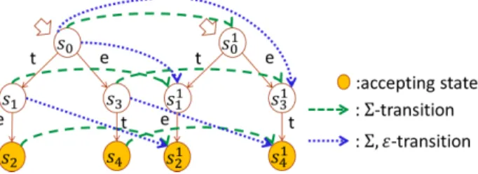
au-Figure 3: Extended Levenshtein Automaton for D =

{“te”, “et”} and k = 1

tomaton for a dictionary. When RD_{= (Σ, S, s}

0, δ, F ) and k are given, we

de-note S0 = S and F0 = F and define the extended Levenshtein automaton LD = (Σ, SL, s0, δL, FL) as

follows:

• We copy all the states and the transition

func-tion k times. We let si _{be the ith copy of s (i =}

1, . . . , k), Si_{consist of s}i_{, and δ}i_{be the ith copy}

of δ. We define SL= S0∪ · · · ∪ Sk.

• s0 is the start state, which is the same state in

RD_.

• We define the transition function δL _{as follows:}

δL(si, a) =          {δi_(si_{, a), s}i+1_}

∪ {δi+1_(si+1_{, b)| b ∈ Σ \ {a}}}

for i = 0, . . . , k− 1,

{δi_(si_{, a)} for i = k,}

for a∈ Σ and

δL(si, ε) ={δi+1(si+1, b)| b ∈ Σ}

for i = 0, . . . , k− 1.

• Let Fi _{be the set of ith copies of states in F}

(i = 1, . . . , k), and FL_{= F}0_{∪ · · · ∪ F}k_.

Figure 3 is an example of the extended Levenshtein Automaton for D ={“te”, “et”}. The extended Lev-enshtein automaton LD _{has many ε-transitions and}

Σ-transitions, so it is inefficient for traversing. Now we make two types of automata which have less non-deterministic transitions than LD_.

3.2

Approach with DFA

Now we make a DFA DLD which is equivalent to

LD_{with subset construction from R}D_{. When R}D_and

k are given, we construct DLD= (Σ, TD_{, t}

0, δD, GD).

The property of each state t ∈ TD _{is following: t is}

represented as a tuple of sets of states (ED0, . . . , EDk)

and we reach t with an input q∈ Σ∗ if and only if we can transform q into w(s), s∈ EDi, i = 0, . . . , k with

i edit operations. We define DLDso as to satisfy the property.

We construct DLD by the following process: 1. Generate the start state t0. ED0 of t0 is {s0}

and EDi of t0 consists of the states reached by

using i ε-transitions from s0. We set the current

state tcurr= t0.

2. Generate a state tchild= (ED′0, . . . , ED′k) from

tcurr = (ED0, . . . , EDk) with a ∈ Σ. ED′i is

recursively defined as follows:

ED′_i =                        {δ(s, a) | s ∈ ED0} for i = 0, {δ(s, a) | s ∈ EDi} ∪ EDi−1 ∪ {δ(s, b) | s ∈ ED′i₋₁, b∈ Σ} ∪ {δ(s, b) | s ∈ EDi, b∈ Σ} for i = 1, . . . , k.

3. If tchild is not a tuple that only consists of ∅,

called non-empty tuple, let tchild be an

accept-ing state if tchild contains an accepting state,

and go to 2 with tcurr= tchild.

4. Generate another tchildfrom tcurrwith another

a∈ Σ and go to 2.

It takes O (

|Σ|2_#TD_|TD_|)_{steps for constructing DL}D_,

where #TD_{is the average number of states of R}D_in

each state of DLD. The number of steps for searching is O(m + #ta), where m is the length of q and #ta is

the number of states of RD in the reached accepting state ta.

Figure 4 is an example of DLD for D = {“te”, “et”}. If we input “tet” into this automaton, we reach accepting state (∅, {s2, s4}) and we obtain the result

“te” from accepting state s2.

3.3

Approach with NFA

Now we make NLD instead of LD _{and DL}D_{. We}

make NLDby removing ε-transitions with subset con-struction and merging all Σ-transitions from one state into one Σ-transition from LD. When RD and k are given, we construct NLD= (Σ, TN_{, t}

0, δN, GN) from

Figure 4: DLD for D ={“te”, “et”}

of states (ED0, . . . , EDk) and we reach t with an

in-put p ∈ Σ∗ if and only if we can transform p into

w(s), s ∈ EDi, i = 0, . . . , k with i edit operations.

We define NLD so as to satisfy the property. We construct NLD by the following process:

1. Generate the start state t0. ED0 of t0 is {s0}

and EDi of t0 consists of the states reached by

using i ε-transitions from s0. We set the current

state tcurr= t0.

2. Generate tchild= (ED′0, . . . , ED′k) from tcurr=

(ED0, . . . , EDk) with a∈ Σ. ED′i is recursively

defined as follows: ED′_i=                  {δ(s, a) | s ∈ ED0} for i = 0, {δ(s, a) | s ∈ EDi} ∪ {δ(s, b) | s ∈ ED′ i−1, b∈ Σ} for i = 1, . . . , k.

3. If tchild is a non-empty tuple, let tchild be an

accepting state if tchild contains an accepting

state, and go to 2 with tcurr= tchild.

4. Generate another tchildfrom tcurr with another

a∈ Σ and go to 2.

5. Generate tsigma= (ED′′0, . . . , ED′′k) with Σ-transition

from tcurr. ED′′i is recursively defined as follows:

ED′′_i =                  ∅ for i = 0, EDi−1 ∪ {δ(s, b) | s ∈ EDi−1, b∈ Σ} ∪ {δ(s, b) | s ∈ ED′′ i−1, b∈ Σ} for i = 1, . . . , k.

6. If tsigma is a non-empty tuple, let tsigma be an

accepting state if tsigma contains an accepting

state, and go to 2 with tcurr= tsigma.

Figure 5: NLD for D ={“te”, “et”}

It takes O(|Σ|2_#TN|TN_{|) steps for constructing NL}D_.

The number of steps we need to traverse NLD with q is O ( k3+ km2+∑ t∈Ta #t )

, where m is the length of

q and Ta is the set of accepting states reached with q.

Figure 5 is an example of NLDfor D ={“te”, “et”}. When we input “tet” into this automaton, we reach the states (∅, {s2}), (∅, {s4}) and we obtain the result

“te” from the accepting state s2.

3.4

Practical Implement of the DFA

Without constructing explicitly any automata such as DLD and NLD, we can search for q in D with imitation of the run of DLD. When RD, a query q =

c1· · · cm (ci ∈ Σ for i = 1, . . . , m), and a threshold

integer k are given, we search the result strings as the following manner:

1. Compute the start state t0of DLDfrom RDand

let tcurr= t0 and i = 1.

2. If i = m, output the results from tcurrand finish

this process.

3. Let tcurr = δD(tcurr, ci) and add 1 to i, and

then go to 2. It takes O

(

|Σ|#TD_m)_{steps for searching with}

prac-tical implement of DLD.

4

Experiments

We made two types of experiments to evaluate our methods. One was measuring construction time of the DFA and the NFA, and the sizes of them. The other was comparing the time for searching of our methods to existing methods.

Table 1: Artificial Data

name |Σ| # of strings length of each word

dic 10 3 10 2 or 3

dic 100 26 100 1 – 10

dic 1000 26 1,000 1 – 10

dic 10000 26 10,000 1 – 10

Table 2: Real Data

name |Σ| the # of strings length of each word

dic P ro 4 106 58

dic Lin 95 1,920 1 – 1920

dic En 95 2,247,773

4.1

Data Used in Our Experiment

4.1.1 Artificial Data

As artificial data, we prepared four dictionaries shown in Table 1. Each dataset has 10, 100, 1000, or 10000 strings. Each string has random length as in Table 1, and each character in a string is randomly chosen.

4.1.2 Real Data

We used three types of real data, dic P ro and dic En (Table 2). The dataset dic P ro is a set of promoter gene sequences1. The dataset dic Lin is the set of all suffixes of a speech manuscript in English (the Gettys-burg Address). The length of the manuscript is 1920 including space symbols, and so dic Lin has 1920 suf-fixes, and let the alphabet Σ be the set of characters from “ ” (the space symbol) to ˜ in ASCII code, the code numbers are from 32 to 126. The dataset dic En is a set of words in an English-Japanese dictionary2, and the alphabet is the same as dic Lin.

4.2

Environment

Our environment in this experiment were as follows.

• CPU: Intel Xeon E5-1650 3.50 × 2 • RAM: 128.00 GB

• OS: Windows 7 (64 bit)

1_{https://archive.ics.uci.edu/ml/datasets/Molecular+Biology+}

(Promoter+Gene+Sequences)

2_{Eijiro 8th edition (英辞郎 第八版),}

http://www.alc.co.jp/cnt/eijiro/

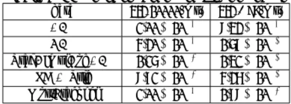
Table 3: Experimental results for the artificial data. TO is timeout, over 3, 600s

data RD _{k DL}D _NLD

time(s) |S| time(s) |TD_{| time(s) |T}N_| 1 0.000 157 0.0000 86 dic 10 0.015 30 2 0.0015 683 0.0000 175 3 0.0235 2,193 0.0 272 1 0.0015 4,002 0.0046 1,513 dic 100 0.015 554 2 0.0233 130,608 0.0078 3,453 3 65.5825 5,014,004 0.038 6,514 1 0.1576 44,512 0.0204 14,074 dic 1000 0.015 4,952 2 0.2387 1,938,692 0.0311 33,461 3 TO 0.334 69.485 1 2.3245 556,334 0.2074 128,505 dic 10000 0.015 43,518 2 3.3352 27,020,846 0.2623 343,338 3 TO 5.001 833,279

Table 4: Experimental results for the real data. TO is timeout, over 3, 600s

data RD _{k DL}D _NLD

time(s) |S| time(s) |TD_{| time(s) |T}N_| 1 0.0499 24,721 0.0354 17,991 dic P ro 0.040 5,880 2 0.425 130,040 0.124 47,444 3 6.629 1,091,688 0.434 112,073 1 42.3837 6,592,244 8.564 4,318,789 dic Lin 3.132 1,090,734 2 TO 53.917 12,072,152 3 TO 182.189 27,260,602 1 TO 166.8626 74,942,58 dic En 6.893 24,699,097 2 TO TO 1 TO TO

We implemented the algorithms in C++ and used gcc 4.8.2 as a compiler with an option “-O3”. We used the library Darts3 _{as an implementation of tries.}

4.3

Experiments of Construction and

Results

We measured the time for constructing DLD and

NLD, and the number of their states|TD_{| and |T}N_|

re-spectively for each artificial dataset and real dataset. We let the threshold k = 1, 2, 3. We constructed the automata 10 times and calculated the average time.

Tables 3 and 4 show the results with the artificial data and with the real data.

Both of the computational time in construction and the number of the states in ELD _{are less than those}

of DLD. |TN_{| is linear to the number of strings in the}

artificial dictionary. |TD| is also linear in the case of small k.

Table 5: Experimental results of the search

data dic 10000(ms) dic P ro(ms) DLD 2.00× 10−3 9.43× 10−3

NLD _{5.30× 10}−3 _{1.68× 10}−1 Prac. Impl. of DLD 1.26× 10−2 1.42× 10−1 LA & Trie 9.82× 10−2 5.37× 10−1 Mor-Fraenkel 2.00× 10−3 1.89× 10−2

4.4

Experiments of Search and Results

In order to evaluate the searching performance of our methods, we compare the time for searching of our methods to that of existing methods. We implement the Levenshtein automaton and trie based method de-scribed in [1] and Mor-Fraenkel method [6]. We used two data, dic 10000 and dic P ro, and let k = 1.

Table 5 is the result. As a result, constructing

DLDmethod takes the shortest time. This is because the constructing DLDmethod just need to transition with the given query. NLDneeds less time than Mor-Fraenkel method for dic 10000, while NLDneeds more time than Mor-Fraenkel method for dic P ro. This is because NLDneeds more and more time for transition when the query is longer and longer.

5

Conclusion and Future Plan

In this paper, we treat the problem of approximate string matching for a dictionary. In order to solve the problem, we take a policy of extending Leven-shtein automata for tries. We define DLD and NLD as the automata for finding strings in the dictionary which approximately match a given query string, and we propose the construction algorithms of DLD and

NLD. The number of steps of both algorithms are lin-ear to the number of strings in the dictionary and the numbers of states in the output automata. Moreover, we propose a searching method imitating the run of

DLD. As the results of the experiments of construct-ing the automata, we can construct DLDand NLDin linear time to the numbers of strings in the dictionary in the case of allowing a few errors. The experiments for searching show that DLD is faster than existing methods. The running time of NLD is faster than the existing methods for short queries, while the ex-isting method is faster than running the NFA for long queries.

As a future plan, we will work on the following items: analyzing the computational complexity of our

method more precisely, comparing the time for search-ing with our methods to existsearch-ing methods more pre-cisely, and applying our methods to other applications on suffix trees.

Acknowledgments

This work was supported by JSPS KAKENHI Grant Number 26280085.

Reference

[1] Boytsov, L.: Indexing Methods for Approximate Dictionary Searching: Comparative Analysis,

Journal of Experimental Algorithmics, Vol.16,

pp.1.1:1.1–1.1:1.91 (2011)

[2] Baeza-Yates, R.A. and Gonnet, G.H.: A fast al-gorithm on average for all-against-all sequence matching, String Processing and Information

Retrieval Symposium, 1999 and International Workshop on Groupware, pp.16–23 (1999)

[3] Jokinen, P. and Ukkonen, E.: Two Algorithms for Approximate String Matching in Static Texts,

Mathematical Foundations of Computer Science 1991, pp.240–248 (1991)

[4] Wang, B., Xie, L, and Wang, G.: A Two-Tire Index Structure for Approximate String Match-ing with Block Moves, Database Systems for

Ad-vanced Applications, pp.197–211 (2009)

[5] Schulz, K. and Mihov, S.: Fast String Correction with Levenshtein-Automata, International

Jour-nal of Document AJour-nalysis and Recognition, vol.

5, pp.67–85 (2002)

[6] Mor, M. and Fraenkel, A. S.: A Hash Code Method for Detecting and Correcting Spelling Errors, Communications of the ACM, vol. 25, is-sue 12, pp.935–938 (1982)