275
On the Orthogonal $L_{1}$ Linear Approximation of PointsPeter Yamamoto*\dagger , Keiko Imai\ddagger and Hiroshi Imai* *Department of ComputerScience and Communication Engineering
Kyushu University, Fukuoka812, Japan \dagger School of Computer Science, McGill University
Montreal, PQ, Canada $H3A2K6$
\ddagger Department of Mathematical Engineering University ofTokyo, Tokyo 113, Japan Abstract
This paper presents algorithms for $app$roximating a set of$n$ poin$ts$ by a $1i_{J1}$ear function, or a
line, that $m$inimizes the $L_{1}n$orm oforthogon$aJ$ distances., The algorithms fin$d$ exact solu tions
based upon geom$e$tric $p$roperties of the proble$ms$ as opposed to approximate $sol$utions based
upon $ex$istingnumerical techniques. The algorithmic complexity oftheseproblems appears not
to $ha\gamma e$ been investiga$ted$, altho$ughO(n^{3})$ naive algorithms can be easily obtain$edb$as$ed$ on
$somesimplech$arac teristics ofoptimal $L_{1}$ solu tions. In this pap er, an $O(n^{1.5}\log^{2}n)$ algori$thm$
is $pr$esented for the unweigh$ted$ orthogon$al$ problem, an$d$ an $O(n^{2})$ algorithm is
$p$resented for $a^{heweightedproblem.An\Omega(n1ogn}tcertainmode1\circ fcomputation.A1_{so,thecomp1exityofsolvingtheo^{1}rthogona1Lprob1emis}^{lowerboundfortheorthog\circ flalLproblemiss_{1}hownunder}$
rela$ted$ to the $cons$truction of the k-belt ofan arrangement oflines.
1. Introduction
Approximating a set of$n$ points in the
plane bya linearfunction,or aline,called
the line-fittingproblem, is a fundamental problem in scientific computing
encoun-tered in many fields, including statistics, econometrics,location theory,and signal-processing. Recently,the line-fitting pro-blem and its variationshave been consid-ered from an algorithmic point of view in those areas. However, the algorithms presented are, for the most part, brute
force and involve enumeration of all possible candidate solutions. Solutions to some of these
$pro$blems,on the other hand, have inherent geometrical propertieswhich havegeneratedinterest
from the area of discrete and computational geometry.
The nature of the problem depends on three factors: the distance function used to measure the distance from a point to a line, the norm of the distance function used, and whether the
distances areweighted by associating a weight to each point. The unweightedcasecorresponds
to the situation where all weights are equal to one. Vertical, $d_{v}$, or orthogonal, $d_{o}$, distances
are commonly used as the distance function (see Figure 1.1), although other measures, such
as the rectangular distance, are also of interest.
Themost frequently usednorm is the $L_{2}$ norm which may be efficiently solvedby theleast
squares method for both vertical and horizontal distances. However, the $L_{2}$ norm is not always
the most appropriate criteria for a “best” fit. The two most popular alternatives are the $L_{1}$ and
the $L_{\infty}$ (or Chebyshev) norms; however, their use in practice has been limiteddue tothe lack of
effcient algorithms (seethe conclusion for abrief historical note). The full paper provides details
276
Megiddo [10] notes that by ap-plying his multidimensional search
technique to the vertical $L_{\infty}$
pro-blem, formulated as a linear
pro-gramming problem, an exact
solu-tion may $b’e$ found in linear time.
Recently, Lee andWu [9] provide op-timal and efficientalgorithmsforthe orthogonal$L_{\infty}$ problemandsomeof
its variations.
Optimal solutions to both the verticalandorthogonal$L_{1}$ problems
are known in statistics $as$ robust
es-timators: the solutions are not
eas-ily influenced (relative to solutions
$totheL_{2}andL_{\infty}prob1ems1iers,ornoise,inthedata/seeFig-byout-$
ure
1.2). For that reason, in appli- Figure 1.2. Effect ofoutliers on optimal solutions.cations in which the data is subject
to error, for example, signal‘ processing, the $L_{1}$ norms may be much more preferable than the
morepopular$L_{2}$ norms. Also, fromthe viewpoint oflocationproblems, theorthogonal $L_{1}$ norm
measures the total Euclidean distance of the points from the line.
The unweighted vertical $L_{1}$ problem may be solved by general numerical approximation
methods, such as the method ofdescent, or it $may$ be formulated as a linear programming
pro-bleminhigher dimensions [3]. [8] notes an $O(n^{3})$ naivealgorithmforfindingan exact solution to
theweighted vertical $L_{1}$ problem basedon characteristic properties ofoptimal solutions. In the caseof the unweighted orthogonal $L_{1}$ problem, [13] presents a numerical algorithm which
corre-sponds to a concavequadratic programming algorithm. [11] presents an$O(n^{3})$ naive algorithm
for finding an exact solution to the weighted orthogonal $L_{1}$ problem based on characteristic
properties of optimal solutions.
Thecomplexity ofthe vertical and orthogonal $L_{1}$ problems appears not to havebeen
inves-tigated from an algorithmic point of view before our work in [8]. The problems differ only by
thedivisor $\sqrt{a^{2}+1}$which converts the vertical distance into the orthogonal distance; however,
the divisor is an important factor in determining the complexity of the problems. [8] presentsa
linear time algorithm for the unweighted vertical$L_{1}$ problem; however, the results in this paper
indicate that algorithms for the orthogonal $L_{1}$ problems lie in a differentcomplexity class.
This paper is concerned with the unweighted and weighted orthogonal $L_{1}$ linear
approxi-mationproblems in the plane. The weighted problem may be stated as follows.
Problem 1.1. The Orthogonal $L_{1}$ Problem. Given a set, $S$, of$n$ poin$ts,$ $Pi\equiv$
$(x;, y_{i})(i=1, \ldots , n)$, in the $(x, y)- plaJ1e,$ $wi$th correspondin$g$ weights, $w;$, find a pair
of valu es (a $b$“), for the parameters $a$ an$db,$ $wh$ich solves the followin$gmin$i-sum
problem:
$\min_{a_{l}b}\sum_{1=1}^{n}w;\frac{|y_{i}-(ax_{i}+b)|}{\sqrt{a^{2}+1}}$
.
The unweighted problemcorresponds to setting all the weights equal to one.
The algorithms presented in this paper find exact solutions to both the weighted and
un-weighted orthogonal $L_{1}$ problems, as opposed to approximate solutions derived by numerical
approximation techniques. The algorithms represent a significant improvementover the
previ-ous $O(n^{6})$ naive algorithms. The complexitiesof the orthogonal $L_{1}$ problems are related to the
construction of the k-belts of an arrangement of lines. The unweighted orthogonal $L_{1}$ problem
is solved in $O(n^{1.5}\log^{2}n)$ time basedupon an algorithmforconstructing k-belts. The weighted
$D_{o}(a, b) \equiv\sum_{i=1}^{n}w;\frac{|y_{i}-(ax_{i}+b)|}{\sqrt{a^{2}+1}}$
.
The absolute value signs may be eliminated by considering the value of the function for fixed
values of the parameters $a$ and $b$
.
For fixed $a$ and $b$, define sets $I_{A}(a, b)$ and $I_{B}(a, b)$ of indicesby:
$I_{A}(a, b)=\{i|y;>ax_{i}+b (i=1, \ldots , n)\}$
and
$I_{B}(a, b)=\{i|y;<ax;+b (i=1, \ldots , n)\}$
.
Note that the above notation may be interpreted as $t$he set of indices of data points $(x;, y;)$
above and below a line defined by $(a, b)$ in the $(x, y)$-plane, or as tbe correspondingset ofindices
of data lines defined by $(-x_{i}, y_{i})$ above and below a point $(a, b)$ in the $(a, b)$-plane.
$D_{o}(a, b)$ may then be written as follows.
$D_{o}(a, b)= \sum_{=:1}^{n}w;\frac{|y_{i}-(ax_{i}+b)|}{\sqrt{a^{2}+1}}$
$= \sum_{1\in I_{\wedge}(a,b)}w;\frac{y_{i}-(ax_{i}+b)}{\sqrt{a^{2}+1}}-\sum_{ii\in I_{D}(a,b)}w;\frac{y_{i}-(ax:+b)}{\sqrt{a^{2}+1}}$
$= \frac{a(X_{B}-X_{A})+b(W_{B}-\dagger V_{A})+Y_{A}-Y_{B}}{\sqrt{a^{2}+1}}$
where
$W_{A}= \sum_{:\in I_{A}}w;$, $X_{A}= \sum_{i\in l_{\Lambda}}w;x;$, $Y_{A}=\sum_{j\in I_{A}}w_{i}y;$,
$W_{B}= \sum_{:\in I_{D}}w;$, $X_{B}= \sum_{i\in l_{B}}w;x;$, $Y_{B}=\sum_{i\in I_{B}}w;y;$
.
Hence,given thevalues of$W_{A},$ $X_{A},$ $Y_{A},$ $YV_{B},$ $X_{B}$ and $Y_{B}$, the value of$D_{o}(a,b)$ can becomputed in constant time.
278
Suppose the values of the above variables are computed for some fixed parameter values $a’$ and $b’$
.
If the next computation is for new values, $a”$ and $b^{u}$, such that theabove-below
relationships of the data points and the lines defined by $y=a’x+b’$ and $y=a”x+b”$ do not
change, then the values of those variablesalso do not change. Hence, theobjective functionfor the parameters $a”$ and $b”$ can be computed in constant time. The aboverepresentation scheme
is used in all the algorithmsfor maintaining the contributionof the datapointsto the objective function.
Morrisand Norback [11] present two characteristic properties of an optimal orthogonal $L_{1}$
problemsolution.
Lemma 2.1. There is an approximate $line$ to the $p$oint set $S$ which minimizes the
orthogon$alL_{1}$ norm an$d$ which$p$asses thro$ugh$ twopoints of$S$
.
Lemma 2.1 suggests an $O(n^{3})$ brute force approach to solving the problem. For each of the
possible
(:)
pairs of points, evaluate thefunction for a line which passes through the pair.Lemma 2.2. The sum of the weights on the optimal $app$roximation line isgreater
than the difference of the
sums
of weigh$ts$ on either side of the line.Both Lemma 2.1 and Lemma 2.2 also hold in d-dimensions and can be solved by
an
$O(n^{d})$-time and $O(n)$-space algorithm. The details will appear in a laterpaper.
Morris and Norback suggest using both properties to find candidate$sol$ution$s$,pairs ofdata
points in the $(x, y)$-plane (or pairs of lines in the $(a,b)$-plane) which satisfy both properties.
They suggest the brute force approach of inspecting each of the possible
(:)
pairs to see if theline defined by the pair satisfies the second property; if so, then compute the $L_{1}$ norm with
respect to the candidate line defined by the pair ofpoints. Clearly, that algorithm is not agreat improvement over computing the $L_{1}$ norm for every possible pair. However, the approach does
raise the question of how many candidate pairs there are and what is the complexity of finding them. That question can be related to the number of k-sets as described below.
Given a set $S$ of $n$ points, a k-set of $S$ is a subset $S’$ such that $S$‘ contains $k$ points and
thereexists a line, $l_{k}$, whichseparates $S’$ from $S-S’$
.
The number of k-sets of aset of$n$points$h$as been shown to have complexities of9$(n\log k)$ and $O(nk^{1/2})[7]$
.
The computation of k-setsisstudied in [6]. In that paper, they introduce the notionof k-belts in the dual plane.
For each point$p$ in thedualplane, let $b(p),$ $o(p)$, and$a(p)$ denote the number of lines which
lie below $p$,
on
$p$, and above $p$, respectively. Clearly $b(p)+o(p)+a(p)=n$ , for all $p$.
Thek-belt, for $0\leq k\leq\lceil n/2\rceil$, of the arrangement of lines in the dual plane is defined as the set
ofpoints $p$ in the dual plane such that $b(p)+o(p)\geq k$ and $a(p)+o(p)\geq k$
.
The O-belt is thewhole plane, and for $k\geq 1$, the k-belt is bounded above and below byan unbounded monotone
polygonal chain. For $n$ odd and $k=\lceil n/2\rceil$, the two boundaries of the $\lceil n/2\rceil$-belt,referred to
as
the median-belt, coincide. The bold line in Figure 2.2(b) represents the median-belt for the
seven lines shown in Figure 2.2 (a).
In the unweighted problem, Lemma 2.2 is just a cardinality problem: the difference in
the number of points above and below the line must not exceed the number of points on the line. The number of candidate lines is related to the number of k-sets, or umedian’-sets since
$k=\lceil n/2\rceil$, of a set of$n$ points in the $(x, y)$-plane. Similarly, the number of candidate lines in
the weighted problem is related to the number of “weighted” k-sets,
or
weighted median-sets, since the line must satisfy the second property which balances the weights equallyon each side ofthe line.3. The Unweighted Problem
In the unweighted orthogonal $L_{1}$ problem, the dual transformationsofthe candidate lines
cor-respond to the vertices of the $\lceil n/2\rceil$-belt, or median-belt (see Figure 2.2). The algorithm
presented below evaluates the function at each of those vertices in order to determine an
op-timal $va|ue$ (the existence is guaranteed by Lemma 2.2). The function evaluations can be
performed in the same amount of time as it takes to construct the median-belt.
The construction of the k-belt of an arrangement, $H$, of $n$ lines can be performed in
$O(b_{k}(n)\log^{2}n)$ time and $O(n)$ space,where $b_{k}(n)$ is themaximum number ofvertices in the $k-$
Figure 2.2.(a) Candidates in $t$he $(x, y)$-plane.Figure 2..2.(b) Candidates in the $(x, y)$-plane.
and $b_{\lceil n/2\rceil}(n)=O(n^{1.6})$
.
The algorithm sweeps the arrangement by a vertical line $L$ from left to right. At $a=-\infty$,
the data line, $l_{m}$, with the median slope also has the median intersection with $L$
.
Let $H_{A}$ bea set of data lines above $l_{m}$ an$d$ similarly $II_{D}$ a set of data lines below $l_{m}$ with respect to the
median intersection point. IIence, the sets $I_{A}$ and $I_{B}$, as defined in Section 2, refer to the
indicesofthe linesin $H_{A}$ and $H_{B}$, respectively, and thevariablesused to maintain $D_{o}(a, b)$ (see
Section 2) can be initialized in linear time.
The algorithm then sweeps the arrangement to find the next vertex on the belt which is the intersection of $l_{m}$ and another data line $l_{A},$ $w$here without loss of generality the line $l_{A}$
is assumed to be in the set $H_{A}$
.
The value of $D_{o}(a, b)$ may $be$ computed at the new vert$ex$in constant time as follows. Subtract $x_{A}$ from $X_{A}$ and $y_{A}$ from $Y_{A}$
.
Add $x_{m}$ to $X_{A}$ and $y_{m}$to $Y_{A}$
.
Those operations take constant time and $D_{o}(a, b)$ may be computed in constant timewith the updated values. The algorithm keeps a pointer to the swept vertex which minimizes
$D_{o}(a, b)$; clearly, such a pointer can be updated in constant time. Thus, each step of the plane
sweepcanbedone without increasing the complexity ofthe k-belt construction algorithm. Since
$O(n^{1.5}\log^{2}n)$ time is spent in constructing the median-belt, the following result is obtained.
Theorem 3.1. The $u$Ilweigh$ted$ orthogonal $L_{1}lin$ear approximation problem for $n$
poin$ts$ can be solved in $O(n^{1.6}1og^{2}n)$ time and$O(n)$ space.
The above algorithm, although eMcient, is still an exhaustive search of all the candidate solutions. Note that the algorithm is for constructing the general k-belt; for at least one value of$k,$ $k=1$ , a more $e$Mcient algorithm, $O(n\log n)$ time, can be obtained by considering the
particular problem. IIence, the authors conjecture that a more efficient algorithm may be
obtainedby considering the particular properties of themedian-belt.
4. The Weighted Problem
In the dual plane, the candidate solutions to $t$he weighted orthogonal $L_{1}$ problem lie on the
boundary of the weighted median-belt of the arrangement, the set of points which are the dual transformations of the weighted median lines in the $(x, y)$-plane. IIence, the complexity of
finding a solution can be related to the number of vertices (due to Lemma 2.2), $n_{w}$, on the
280
Figure 4.1.(a) $\Omega(n^{2})$ Degenerate vertices. Figure 4.1.(b) $\Omega(n^{1.6})$ Non-degenerate vertices.
The complexity of $n_{w}$ depends on how a vertex of the median-belt is defined. A vertex
can $be$ described as either any point on the boundary of the weighted median-belt which is
incident to $mo$re than one lineof the
arrangement.
(called degenerate vertices), or any point onthe boundary of the weighted median-belt whose lncident boundary edges are distinct (non de-genera$te$vertices) (see Figure $4.1(a),(b)$). Note that the nondegenerate vertices are a subset
ofthe degenerate vertices.
Since the weighted median-belt is an x-monotone chain, the number of vertices can be
bounded by results for monotone chains. The number of degenerate vertices is $\Omega(n^{2})[14]$ (see
Figure $4.1(a))$
.
The number ofnon-degeneratevertices is $\Omega(n^{1.6})[12]$ (seeFigure 4.1(b),$n=$$\sqrt{k}$, shaded area has $k^{2}$ vertices); although an (unknown at the time of printing) improvement
to this lower bound has been reportedly made by R. Cole and J. $Mat_{ou}g_{ek}[4]$
.
Note,however, thatnot all x-monotone chainsare weightedmedian-belts. In thecaseof the example for the degenerate bound, legal weight $as$signments (bold numbers)
can
be given to thelines, however, the particular example given for the nondegenerate bound cannot be assigned weights such that the chain becomes a weighted belt.
Thegeometry of the (unweighted) median-belt and of the weightedmedian-beltcan be quite
different. In the unweighted case, themedian-belt only hasnondegenerate vertices since the belt
switches lines at every intersection. In the weighted case, however, the weighted median-belt may not switch at an intersection if the current edge has a relatively large weight.
An algorithm based only on the properties given by Lemma 2.1 and Lemma 2.2 must check the objective function at all degenerate vertices. Hence, the complexity of applying the k-belt construction algorithm, mentioned above, to the weighted problem is in $O(n^{2}\log^{2}n)$
.
However, the weighted orthogonal $L_{1}$ problem can be solved in $O(n^{2})$ time by the following
“efficient” brute force algorithm.
An optimal solution is found by performing an $O(n^{2})$ time, $O(n)$ spac$e$ plane sweep as
described in [5]. Note that thisplane sweepdiffers from the planesweep algorithm used for the
unweightedcase; the plane sweep used above only computespoints of interest in order from left to right, whereas the plane sweep used here reports all $O(n^{2})$ verticesof the arrangement in an
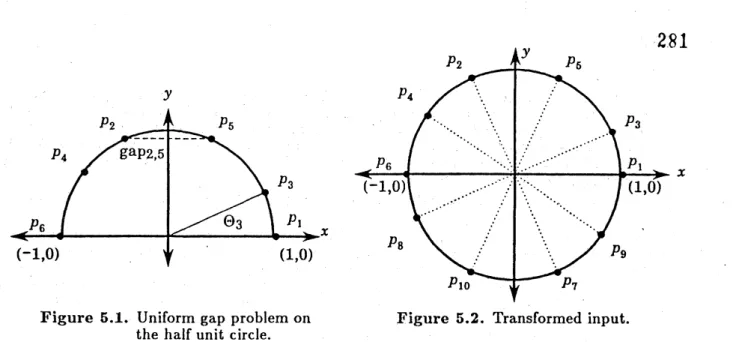
Figure 5.1. Uniform gap problemon Figure 5.2. Transformed input. the half unit circle.
First, note that the leftmost edge ofthe weighted median-belt can be determined in linear time. Second, the plane sweep algorithm insures that, theoretically, each vertex is incident to only two lines; hence, determ.iningwhether a switch to a new line should take place at a vertex of the belt can be decided in constant time by maintaining $D_{o}(a, b)$ as described in Section 2.
Third, since the next event vertex in the sweep is identified by its incident edges (lines), the vertex can $be$ tested to see ifit is on the belt by simply comparing the current edge ofthe belt
to the incident lines in constant time.
Since the plane sweep is performed in $O(n^{2})$ time and the extra cost to maintain the
weightedmedian-belt and the function $D_{o}(a, b)$ is$O(1)$ time for each vertex,anoptimal solution
may be found in $O(n^{2})$ time. The algorithmis called an efficientbrute force algorithm since the
computations areperformed efIiciently, reducing $t$he complexity ofa pure brute force search by
a factor of$O(n)$
.
Alsonote that the above algorithm implies that the algorithm for constructingk-belts used in the unweighted problem is not, at least in onecase, the mostefficient algorithm
forcomputing weightedk-belts.
5. $\Omega(n\log n)$ Lower Bound
This section provides an $\Omega(n\log n)$ lower bound for the orthogonal $L_{1}$ problem under the
al-gebraic computation tree model [2]. (Due to $sp$ace limitations not all the proofs are included
in this paper). First, the lower bound of the complexity of a certain uniform gap problem of
$n$ points on a circle is shown to $be$ in 9$(n\log n)$ under the algebraic computation tree model.
Second, that uniform gap problem is reducedto theunweighted orthogonal $L_{1}$ problem in linear
time, thus proving an $\Omega(n\log n)$ lower bound for the orthogonal $L_{1}$ problem.
The uniform gap problem on the unit circle is defined as:
Problem 5.1. Uniform Gap Problem on the (Half) Unit Circle. Given
$m+1$ poin$tsp_{1},p_{2},$ $\ldots,$$p_{m},p_{m+1}$ on the unit circle $x^{2}+y^{2}=1$ such that $p_{1}=(1,0)$,
$p_{m+1}=(-1,0)$ and the y-coordinates of points $p;(i=2, \ldots , m)$ are positive (see
Figure 5.1), the uniformgap problem on the unit circle answers whether the$d$istances
of every consec$u$tive pair of poin$ts$ are equ$al$ when these $m+1$ poin$ts$are arranged in
increasingorder of their polar angles.
Denote the $(x, y)$-coordinates of point $p$
:
by $(x;, y;)$,where $x_{1}=1,$ $x_{m+1}=-1$ and $y:\geq 0$.
For a permutation $\sigma$ on $\{$2,
$\ldots$,$m\}$, define $W_{\sigma}\subset Il^{m-1}$ by
$W_{\sigma}=,$ $\{(x_{2}, \ldots, x_{m})\in It^{m-1}|1=x_{1}>x_{\sigma(2)}>x_{\sigma(3)}>\cdots>x_{\sigma\langle m)}>x_{m+1}=-1$,
$(x_{\sigma(i+1)}-x_{\sigma(i)})^{2}+(\sqrt{1-x_{\sigma(:+1)}^{2}}-\sqrt{1-x_{\sigma(:)}^{2}})^{2}=\epsilon^{2}\}$ ,
where $\sigma(1)=1$ and $\sigma(m+1)=m+1$
.
Define $W\subset R^{m-1}$ by $W= \bigcup_{\sigma}W_{\sigma}$ where the union is 728,2
taken overall permutations$\sigma$ on $\{$2,
$\ldots$,$m\}$
.
Then the answerfor the uniform gap problemforpoints $p_{1},$ $p_{2},$$\ldots,$$p_{m+1}$ is yes if and only if $(x_{2}, \ldots, x_{m})\in W$, which implies that, by Ben-Or’s
theorem [2], a $10$wer bound for thecomplexity of the uniform gap problem under the algebraic
computation tree is 9$(\log\# W)$ where $\# W$ is the number of connected components of W. $\# W$
can be shown to be equal to $(m-1)!$, hence, the following result holds under the algebraic computationaI$mo$del of Ben-Or.
Lemma 5.1.. The complexity of the uniform gap problem on the unit $c$ircle is $\Omega(m$
$\log m)$
.
Next, the input for the uniformgap problemona circle is transformed,in linear time, toan
input for the orthogonal linear $L_{1}$ approximation of points. Given the points $p_{1},p_{2},$$\ldots,$$p_{m+1}$
of the uniform gap problem, assume that, without loss of generality, $0=\theta_{1}<\theta_{2}<\cdot\cdot:<\theta_{m}<$
$\theta_{m+1}=\pi$, where $\theta_{:}$ denotes the polar angle of $Pi$
.
For each$Pi$ $(i=2, \ldots , m),$ $co$nstruct the
point $Pi+m$ on the unit circlewhose polar angle $\theta_{i+m}$ is $e$qual to $\theta_{j}-\vdash\pi$ (see Figure 5.2). The
set, $S$, of $n=2m$ points
$p_{1},p_{2},$ $\ldots,p_{n}$ is then used
as
theinput for theorthogonal $L_{1}$ problem.The transformation is then completed by showing the following result.
Lemma 5.2. The minimum objective function value of the orthogonal $L_{1}$ linear
approximation for the set $S$ of poin$ts$is at most 2$\cot\frac{\pi}{n}$, and is 2$\cot\frac{\pi}{n}$ if an$d$ only if
the answerfor the
uniform.
gap problem of$po$in$tsp_{1},$ $p_{2_{1}}\ldots,p_{m},p_{m+1}$ is yes,The proof is developed as follows. For the orthogonal linear $L_{1}$ approximation problem, it
is known that there is an optimal approximation line such that the line passes twopoints among thegiven pointsand $|N_{A}-N_{B}|<N_{O}$whe$reN_{A},$ $N_{B}$ and $N_{O}$ are the numbers of points above,
below, and on the line [11]. By the definition of the transformed problem, there is an optimal approximation line among the $m$ lines $l$; connecting points
$p$
:
and $p_{1^{\}}+m}(i=1, \ldots, m)$.
Thefunction value of$\iota_{:}$, the summationof $t$he orthogonal distances from points $Pj$ $(j=1, \ldots , n)$ to
$l_{i}$
,
is given by$\sum_{j=1}^{n}|sin(\theta_{j}-\theta_{i})|$
.
(1)Hence, the minimumfunction valueof the orthogonal linear $L_{1}$ approximation for $S$ isgiven by $\min_{i=1,\ldots.m}\sum_{j=1}^{n}|\sin(\theta_{j}-\theta_{i})|$
.
(2) We are considering to maximize (2) for $0=\theta_{1}<\theta_{2}<\cdots<\theta_{m}<\pi$ and $\theta_{i+m}=\theta_{:}(i=$$1,$$\ldots$,$m$). However, this is
an
optimization problem of maximin type, and rather difficult tohandle directly. Instead,we will consider to maximize
$\sum_{:=1}^{m}\sum_{j=1}^{n}|\sin(\theta_{j}-\theta_{i})|$
.
(3)Here, observe that the function values for lines $l$; are the same when the set $S$ of points are
uniformly placed on the circle. Hence, if (3) is maximized when and only when the set $S$ of
points are uniformly placed, then (2) is maximized only in the
same
uniform case.Let us prove that (3) is maximized when andonly when the set $S$ ofpoints are uniformly
placed. (3) is further expressed
as
$\sum_{1=1}^{m}\sum_{j=1}^{n}|\sin(\theta_{j}-\theta_{i})|=2\sum_{1=1}^{m}\sum_{j=i+1}^{:+m}\sin(\theta-\theta)=2\sum_{k=1}^{m}(sin(\theta-\theta_{j}))$
For any $k=1,$$\ldots$ ,$m$, we have
$0<\theta_{i+k}-\theta:<\pi,$$\sum_{=:1}^{m}(\theta_{i+k}-\theta:)=k\pi$
.
Since $\sin x$ is strictly
concave
on the interval $[0, \pi]$, we haveand the equality holds if and only if all $\theta;+k-\theta$; $(i=1, \ldots , m)$ are equal. All $\theta_{i+k}-\theta$;
$(i=1, \ldots , m)$ are equalfor any$k=1,$$\ldots$,$m$ if and only if all $\theta_{i+1}-\theta;(i=1, \ldots , m)$ are equal.
Hence, (3) is maximized when and only when the set $S$ ofpoints are located uniformly on the
circle.
When
the set $S$ of points are placed uniformly, thefunction value ofthe orthogonal linear$L_{1}$ approximation is expressed by
$\sum_{j=1}^{n}|\sin\frac{j\pi}{m}|=2\sum_{j=1}^{m}\sin\frac{j\pi}{m}=2\cot\frac{\pi}{2m}=2\cot\frac{\pi}{n}$
.
Thus, we$h$ave shown Lemma 5.2.
Using the above lemmas, the following result provides a lower bound for the orthogonal $L_{1}$
problem.
Theorem 5.1. Under the algebraic computation tree model, the complexity of the orthogonal$L_{1}$ linear approximation of$n$ pointsis $\Omega(n\log n)$
.
This result is mainly of interest to the unweighted orthogonal problem since the actual bound for the algorithm presented above is in $O(b_{k}(n)\log^{2}n)$, where $b_{k}(n)$ is the number of
k-sets of$n$ points $(k=\lceil n/2\rceil)$
.
As mentioned abov$e$, the bounds for $b_{k}(n)$ are in $\Omega(n\log k)$ and $S(o\Omega t(r(nank_{1^{1}og}uss^{6})_{n}[7|_{fork=\lceil n/2\rceil)^{O(n^{2}),respectively,fork=\lceil n/2\rceil),butErd\overline{o}s,Lov\acute{a}sz,Simmons,and}}^{\Omega(n\log n)and}conjecturethat.theupperboundisactuallyc1osertothelowerboundof\Omega\{n\log k)$6. Conclusion
Several results were given concerning the computation and analysis of the unweighted and weighted orthogonal $L_{1}$ linear approximation problems. The results are significant from
theo-retical, practical, and historical viewpoints.
The results are of interest from a theoretical viewpoint since th$ey$ relate the complexities
of the problems to k-sets and k-belts. The complexities of those problems is an open problem in combinatorial geometry. The results presented here motivate further improvements on the
bounds for the number ofvertices in a k-belt. Anotheropen problem is an improved algorithm
for constructing the median belt.
The results are of practical interest since the algorithms $p$rovide efficient algorithms for
solvingthe most popular forms ofthe $L_{1}$ approximation problem. The results are ofparticular
interest for the linear facility problem and the linear regression problem since the algorithms
provide practical and efficient alternatives to the currently used methods (for example, the $L_{2}$
and $L_{\infty}$ approximations).
The results presented here, and also in [8], are of historical interest since this is the last of the three most popular $L_{p}$ approximation problems $(p=1,2, \infty)$ to succumb to efficient
algorithms. [3] notes that alternative criteria to the $L_{2}$ norm have been investigated since the
mid-1750s when R.J. Boscovitch proposed a geometric method for solving a special case of
the $L_{1}$ approximation problem. Interestingly enough, the efficient algorithms for both the $L_{1}$
and the $L_{\infty}$ problems have been derived from applying basic paradigms used in computational
geometry.
’
Continuing research includes the $L_{1}$ problem in higher dimensions, which is of particular
interest to econometricians since they often consider the linear and non-linear $L_{p}$ problems in
higher dimensions [$1|$
.
Solutions to those problems under parallel processing models is alsobeing considered. Furthermore, the paper has raised some questions about the complexity of computing
median-belts
and weighted median-belts.284
Acknowledgements
The authors would especially like to acknowledge the contributions and references provided by Emo Welzl while he was visiting Kyushu University. The authors are indebted to Professor YahikoKambayashiofKyushu University forsupplyingaproductiveresearch environment. The firstauthor acknowledges the support of a JapaneseGovernment (Monbusho) Scholarshipunder
which this research is being carriedout.
References
[1] G. Appa and C. Smith: On $L_{1}$ and Chebyshev estimation, Mathematical Programming. $5$
(1973),
73-87.
[2] M. Ben-Or: Lower bounds for algebraic computation trees. Proc. 15th ACM Symp. oIl Theory of Computing, 1983, $8t\vdash 86$
.
$|\begin{array}{l}345\end{array}|$
VR.
$ColeandJ.Matou8ek,resultcommunicatedbyE.\dot{W}Chv\acute{a}talLinearprogramning.FreemanPress,l983$
elzl.
H. Edelsbrunner and L.J. Guibas: Topologically sweepingan arrangement, Digital Systems
Research Center, April, 1986.
[6] H. Edelsbrunner and E. Welzl: Constructing belts in two-dimensional arrangements with applications. SIAMJ. Compu t., 15 (1986), 271-284,
[7] P. Erd\={o}s, L. Lovkz, A. Sirnmons and E. G. Straus: Dissection graphs of planar point sets. In A SurveyofCombinatorial Theory“ (J. N. Srivastava et al.,eds.), North-Holland, 1973, 139-149.
[8] H. Imai, K. Kato, and P. Yamamoto: A linear time algorithm for linear $L_{1}$ approximation
of points, Kyushu University Technical Report $cscE-87- C30,$ $A_{l1}gust$, 1987.
[9] D.T. Lee and Y.F. Wu: Geometric complexity ofsome location problems. Algorithmica, 1
(1986), 193-211.
[10] N. Megiddo: Linear programming in linear time when the dimension is fixed. J. A CM, 31
(1984), 114-127.
[11] J. G. Morris and J. P. Norback: A simpleapproachto linear facility location. Transportation
Science, 14 (1980), 1-8.
$|\begin{array}{l}1213\end{array}|M.Sharir,resultco.mm\dot{u}nicatedbyEWelzlHSp\tilde{a}thandG.AWatson:Onorthogonal$
linear $L_{1}$ approximation, Numer. Math., 51
(1987), 531-543.