立命館学術成果リポジトリ

(1)

Ritsumeikan Asia Pacific University Graduate School of Asia Pacific Studies

International Cooperation Policy Laboratory of Environmental Geoscience

Master Thesis

Estimating CO

2

Sequestration by Forests in Oita Prefecture, Japan,

Combining LANDSAT ETM+ and ALOS Satellite Remote Sensing Data

Kotaro Iizuka

(Student Number 51210012)

January 2012

(2)

i

List of Figures

Figure 1. Changes in CO2 emissions from 3 targeted sectors in Oita Prefecture, with 2002 as the reference year (100%). ... 1 Figure 2. Location of the study area (Oita Prefecture, Japan). The enlarged image of Oita Prefecture with its administrative units (cities, towns and villages) is shown on the right. ... 4 Figure 3. The analysis flowchart. ... 6 Figure 4. The LANDSAT ETM+ SLC-off product (Dec. 30, 2006). Performance of the gap fill, before (on the left) and after (on the right). ... 8 Figure 5. The vegetation map (National Survey on the Natural Environment) published by the Ministry of Environment. Part of a region at the study area. ... 13 Figure 6. Overall flowchart of the fuzzy accuracy assessment to modify the conventional error matrix to the fuzzy error matrix. ... 15 Figure 7. Forest Tree Age growth curves (Ishii, 2007). Different forest types in multiple locations from Vietnam, Thailand and Japan. The blue line shows the Japanese Sugi (Cedar) Forests growth curve. ... 19 Figure 8. Regression analysis between the solar illumination (cos i) as x-axis, and the radiance value as y-axis for (a) band 1 (b) band 2(c) band 3(d) band 4(e) band 5 and (f) band 7. ... 22 Figure 9. Original near-infrared band (band 4) image (left) and IRC corrected image (right) in radiance over the study area. ... 23 Figure 10. Extraction of Oita Prefecture for LANDSAT ETM+ (a) band 1 (b) band 2 (c) band 3 (d) band 4 (e) band 5 (f) band 7 and PALSAR (g) HH (h) HV. ... 24 Figure 11. Cluster image produced by the ISOCLUSTER module. ... 25 Figure 12. Signature comparison between land cover types. It is the mean radiance value taken from the pixels where the training sites were constructed. 1 to 7 is the May data mean value from band 1 to 7, while w1 to w7 is the December data mean value from band 1 to 7. ... 26 Figure 13. The final output of the land cover map. ... 27 Figure 14. The sigmoidal membership function produced using a cosine function. The points a to d (along the x-axis) represents the inflection points governing the shape of the curve for (a) monotonically increasing shape and (b) monotonically decreasing shape. ... 31 Figure 15. Original NDVI image of the study area on the left, and the reclassed NDVI image on the right. The range of NDVI is compatible with the Sugi tree ages. ... 35 Figure 16. Stem Volume Map of the study area (m3/ha). ... 37 Figure 17. Stem volume as a function of tree age. The Sugi (Cedar) tree age curve on the top and Saw Tooth Oak on the bottom (Oita Prefecture). The growth of stem volume varies among different regions of the study area. ... 38

(5)

iv

List of Tables

Table 1. The questions of the weighting factors. The questions are separated into two, one is the general and the other is the class specific. The general has the general issues which would lead to an error as a general thing, while the class specific will gives questions that focus on each land features. ... 17 Table 2. Computed haze values: Lh (measured in Wm-2 μm-1 sr-1). ... 21 Table 3. Land cover classes. Left = Original output; Right = Final product. ... 28 Table 4. Accuracy of the land cover map from the classification process, on the combination

of multiple images with Type A = 12 class and Type B = 10 class. ... 28 Table 5. Error Matrix showing the reference data versus the image classification. ... 29 Table 6. The scores per category for the accepted classes from the questions. ... 30 Table 7. List of the VCI value used in the fuzzy membership function, and the average

fuzzy value computed for each of the classes of the classified map and the reference map. ... 31 Table 8. Each value represents the fuzzy value computed from the VCI for the accepted

category given by: Average Fuzzy Value (Reference) × Average Fuzzy Value (Classified). ... 32 Table 9. The Probability of Chance Encounter (%) is computed to each of the categories

which were accepted, by adding the scores from the questions and the value from the fuzzy set function. The percentages of the sample points in that category will be counted for the overall accuracy and for both producers and users accuracy. ... 32 Table 10. Fuzzy Error Matrix following the same methodology as traditional error matrix

with the following additions: Non-diagonal cells in the matrix contains accepted and poor. While the numbers in the accepted are considered a “match” for estimating fuzzy accuracy, the numbers in the poor was considered as an error. The fuzzy overall accuracy is estimated as the percentage of sites where the acceptable reference labels matched the classified label. ... 33 Table 11. CO2 sequestration by each forest types of the study area. ... 34 Table 12. CO2 sequestration of the Sugi-Hinoki forest area per tree ages. ... 36 Table 13. CO2 sequestration of coniferous and deciduous broad leaf forests per tree age. ... 39

(6)

v

Abstract

Estimation of CO2 sequestration by the forests of Oita Prefecture, Japan, was implemented. LANDSAT ETM+ (May 25, 2002 and Dec 30, 2006) and ALOS PALSAR (Sep 15, 2009 and Oct 14, 2009) satellite remote sensing data of the study area were acquired and were analyzed with IDRISI Andes/Taiga GIS software platform. Hybrid classification was performed with a maximum likelihood method for producing a detailed land cover map and calculating the total area of the forests (coniferous, deciduous broadleaf and evergreen broadleaf forests). First, CO2 sequestration for each forest types was calculated using the sequestration value per unit area then multiplying with the total forests area, resulting in 6.6 MtCO2/yr in total. Second, for a deeper analysis, the stem volume of the forested area was estimated by using the PALSAR image to find out the tree age for each forest types in order to estimate accurate sequestration. Coniferous and deciduous broadleaf forests were classified into categories per ages and the estimation was made resulting in 2.9 MtCO2/yr and 0.3 MtCO2/yr for coniferous and deciduous broadleaf forests, respectively. The results have shown the importance of considering not only the forest type, but the tree age for estimating more precise CO2 sequestration to prevent overestimation of the forests capacity.

要約

本研究は、大分県の森林が持つ二酸化炭素固定量の算定を目的にしている。 LANDSAT ETM+ (2002 年 5 月 25 日と 2006 年 12 月 30 日) と ALOS PALSAR (2009 年 9 月 15 日と 2009 年 10 月 14 日) 衛星リモートセンシングデータを取得し、GIS ソフトウェア IDRISI Andes/Taiga を用いてすべての分析を行った。ハイブリッドクラシフィケーションに最尤法を用いることで、詳細な土地被覆図の作成を行い、林種別（針葉樹林、落葉広葉樹林、常緑広葉樹林）の総面積を計算した。二酸化炭素固定量の算定は、単位面積当たりの固定量を森林域の面積とで乗じることにより算出した。結果、大分県は全体で 6.6 MtCO2/yr 固定することが分かった。さらに深い分析のために、 PALSAR を用いた材積の推定を実施した。この材積を用いて林種別の森林域を、それぞれの林齢毎の範囲に再分類した。再分類した後、林齢毎の固定量を利用し二酸化炭素固定量を再計算した。結果、針葉樹林は 2.9 MtCO2/yr 、落葉広葉樹林は 0.3 MtCO2/yr を固定することが分かった。これより分かったことは、詳細な土地被覆図の作成による樹種の判別と、樹種毎の林齢を考慮することで過大評価することを避け、より精確な二酸化炭素固定量を算定できるということである。

(7)

1 1. Introduction

1.1. Research Background

Global Warming is considered as one of the most crucial environmental issues in the 21st century. Many research and conferences have been held to emphasize the importance of this issue and associated problems, and many nations are working together on policies if not for preventing the problem, but at least for mitigating its impacts (Hewitt & Jackson, 2003; Chiras, 2006). Japan, is one of the top nations which is involving in many activities related to this issue, and the Kyoto Protocol (adopted at the Kyoto Conference in 1997) has provided a new approach to finding solutions (UNFCC, 1998). Clean Development Mechanism (CDM), Emission Trading, Joint Implementation (JI) and Carbon Sink are the main Kyoto Mechanisms, and among them carbon sink is very important in the current research context, as 68.9% of lands in Japan is covered by forests (OECD, 2004). Japan is considering the forests to be the top candidate for its CO2 reduction process (Ministry of Economy, Trade and Industry (METI), 2005). Many prefectures in Japan have done research about the forests carbon sequestration and have come up with policies for the implementation of reducing CO2. However, some prefectures have not yet been involved in such processes that focus on CO2 reduction through carbon sink although they have a great amount of forest cover. Oita Prefecture is one of them.

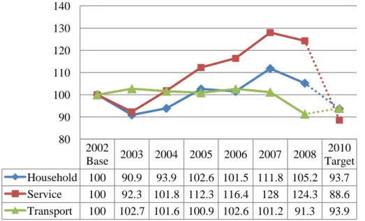
Oita Prefectural Government has so far focused on energy conservation as the main mechanism for effectively reducing CO2 (Oita Prefecture Global Warming Measure, 2006). The Oita Prefecture’s global warming measure implementation has started in 2005, aiming at reducing energy consumption and wastes, and introducing more energy-efficient systems (co-generation system). The results of this approach (Figure.1) do not look so effective at all.

Figure 1. Changes in CO2 emissions from 3 targeted sectors in Oita Prefecture, with 2002 as the reference year (100%) (Oita Prefecture Global Warming Measure, 2010). 2002 Base 2003 2004 2005 2006 2007 2008 2010 Target Household 100 90.9 93.9 102.6 101.5 111.8 105.2 93.7 Service 100 92.3 101.8 112.3 116.4 128 124.3 88.6 Transport 100 102.7 101.6 100.9 102.6 101.2 91.3 93.9 80 90 100 110 120 130 140

(8)

2

It is thus time to reconsider the measure and the tools used by the Prefectural Government for the implementation of this regulation to actually make a step forward to achieve the goals. We have to note that Oita Prefecture has not focused on reducing CO2 through the concept of carbon sink and depending strongly on the energy efficiency which was mentioned above, showing that it is not making much progress towards the goal. The reason for this is more likely because of the lack of sound scientific data needed for objective decision making about which process to use for effectively implementing the policy in the long term.

1.2. Review of Previous Works

Traditional methods of estimating carbon/CO2 through a site-based method (Tadaki & Hachiya, 1968; Bird, 2010) or using eddy covariance flux tower are sometimes expensive, time consuming and limits the coverage of the area. Even to expand the area or implementing continuous monitoring will be more costly and time consuming. Remotely sensed satellite observations have provided the scientists with an alternative method of the way to study the Earth’s nature (atmosphere, vegetation, etc.). On the study of vegetation it has been demonstrated that the reflectance of the wavelength (red, green, infrared) radiation contains considerable information about plant biomass (Tucker, 1979), leading to the extraction of vegetation information and giving us the possibility of monitoring at lower costs and less time. Today, with further advancement of research, it is a common application not only even to produce maps to categorize the land cover type of the surface for allocating and managing the Earth’s resources (Lo & Choi, 2004) but to analyze the changes and its impacts for future developments (Xiuwan, 2002). The remotely sensed method for evaluating the carbon/CO2 sequestration have been implemented in various ways, and one is to use the land cover information to combine with the averaged carbon sequestration value of different land cover types to estimate regional sequestrations (Janssens et.al, 2003). The strength of using land cover information based on remotely sensed images is to cover regional or even global scales of the area and also it can observe sites that are difficult to access when on the ground. Moreover it allows implementation of continuous monitoring of the area for analyzing the changes of the land cover. However, it is important to determine not only the types of land cover but also the differences of the tree age can result in a big difference in the estimation (Turner et.al, 2004). The estimation implemented in Japan is more concerned at the continental scale (whole Japan) which focuses mostly at identifying the forests to the natural and the planted forests. Hiroshima & Nakajima (2006) has focused on the potential carbon sinks in Japanese plantation forests during the first commitment period of the Kyoto Protocol. They have estimated that the private planted forests were expected to sequester 8.16-8.87 MtC/yr, depending on the different scenarios of the forest management based on silvicultural practices, employing subsidies and forest workers’ wages as predictor variables. Sasaki & Kim (2009) has estimated potential sequestration of the forests in Japan and the eligible sequestration under the condition of the Marrakesh Accords. Using the land use model and carbon stock growth model, it has been estimated that the forests in Japan is likely to sequester 20.1 MtC/yr (planted forests: 15.3 MtC/yr, natural: 4.8 MtC/yr), and in the conditions under the Marrakesh Accords,

(9)

3

it is estimated at 10.2 MtC/yr (planted forests: 7.3 MtC/yr, natural: 2.9 MtC/yr). Few studies estimates the potential of the sequestration by the forests in Japan and not many considers to perform an analysis to look through in a local or regional scale focusing more on detailed forest types, which can be understood because the Kyoto Protocol consists at the national level so many studies estimates at that scale. However, in the case of estimations performed by those authors mentioned above are based on a modeling while the information of where and how much those resources exist is not considered, which is not good because it won’t give a further information of then how to make decision for treating those resources. It must also take in consider that the forests are more diverse than just a natural or planted forests. Thus it must be analyzed more on a local or regional scale locating precise and detailed classes of the forests types or the tree types for a realistic estimation of the sequestration, because tree types and even tree ages makes differences in sequestration (Tadaki & Hachiya, 1968; MAFF, 2010). After locating the precise information of the forests, we will be able to estimate the true value of the forests capacity. Once this information is obtained, it will become strong information which can be provided for important decision making on forest management and so on. To plan for future developments and taking decision for actions, the status and location of resource is a critical issue to effectively manage those resources over time.

1.3. Research Objective

The objective of this research is to re-assess the estimation of CO2 sequestration by forests covers in Oita Prefecture based on precise evaluation of forests extents in Oita. This will make it possible to quantitatively estimate their potential storage capacity, and therefore, maximize the usage of this environmental resource as a CO2 sink. These findings will help Oita Prefecture devise better scenarios for mitigating the global warming issue. Local and regional scale analysis of the land cover and estimation of CO2 sequestration will eventually contribute to the updated information of Japan’s CO2 reduction target achievement.

2. Study Area and Data Sets

2.1. Oita Prefecture

The research area, Oita Prefecture, is located on the Kyushu Island at the southwestern part of Japan (Figure.2), between 130.50° E and 132.11° E, 32.43° N and 33.44° N, with a total land area of 6,339 km2. Official figures show that 4540 km2, which make 72 % of lands, are covered by forests (Oita Prefecture Forestry Figures, 2003).

Oita Prefecture is surrounded by several mountains ranges, up to 1758 m in altitude. Climatic conditions divide the prefecture in two main areas: (1) the area effected by the monsoon winds coming from the coast of the Japan Sea, and bringing in large amounts of rainfall and large number of rainy days in winter, and (2) the area characterized by large amounts of rains in summer resulting from the moisture flowing in from the Pacific Ocean, and by dry and fine weathers in winter. The dynamic meteorological factor of these very wet climate conditions

(10)

4

results annual rainfall in Oita Prefecture ranging from 1500~1600 mm over coastal areas, to 2500~3000 mm in the mountainous areas.

Figure 2. Location of the study area (Oita Prefecture, Japan). The enlarged image of Oita Prefecture with its administrative units (cities, towns and villages) is shown on the right.

2.2. Data Sets

2.2.1. Satellite Data

We have obtained four main data sets of satellite data in order to achieve for our analytical objectives. Two optical satellite data sets from the LANDSAT ETM+ with 30 m spatial resolution published by United States Geological Survey (USGS) and two microwave satellite data sets from the ALOS PALSAR published by Japan Aerospace Exploration Agency (JAXA). The selection of the optical satellite data were done by considering the following two critical issues. First, we had to choose a cloud free image for analysis. In fact, finding a cloud free scene is a general issue for all the researchers using optical satellite remote sensing images: clouds block the solar radiation from reaching the ground rendering the covered area unavailable for the observing platform. Second, the Scan Line Corrector (SLC) failure that occurred after May 31, 2003 makes the LANDSAT ETM+ line of sight tracing a zigzag pattern along the satellite ground track. As a result, imaged areas are duplicated, with widths increasing towards the scene edge (USGS, 2010). Although the ETM+ is continuing to acquire image data which are available for downloading at the USGS webpage, a gap fill has to be performed in order to correct the image to become usable for analysis. We needed to choose a winter season data for the purpose of our analysis. The data is preferable to choose the same year data, but because of the issue of the cloud cover this could not be fulfilled, and later year

(11)

5

data was chosen and because of that the issue of the gap fill needed to overcome. As a result, we selected the cloud free LANDSAT ETM+ image captured on May 25th, 2002 and Dec 30th, 2006 as the best fit for our analysis purposes.

For the microwave data, we have chosen the level 1.5 product of ALOS PALSAR L-band data of Sep 15th, 2009 and Oct 14th, 2009 for to cover the study area with an ascending Fine Beam Dual (FBD) Polarization, off nadir angle of 34.3 degree, 12.5 m ground range pixel spacing specification. A mosaic image of the study area is produced using these data sets.

2.2.2. Ground Truth

In order to verify the contents of the pixel on the images, we need to obtain a reference data to compare what is there in reality. Here, we have obtained three data to help determine the contents of the surface. One is The National Survey on the Natural Environment (6th and 7th Surveys, performed from 1999 and later on), which is published by the Ministry of Environment, Japan, provides the status of lands, surface waters and coastal areas all over the nation. The survey results are compiled and published in the form of written reports, maps, etc. The vegetation map so provided is utilized for identification of specific land-use/land-cover (LU/LC) sites for ground truth training data needed for land features classification and for the accuracy assessment of the classified images. Second, is the ALOS PRISM Panchromatic data with 2.5 m spatial resolution at nadir. This data is used with the combination of the vegetation map for the confirmation of the land surface. Third, a field observation was performed to collect ground truth data of the sites and identify the land features of the sites.

2.2.3. Digital Elevation Model (DEM)

A digital model of a terrains surface is obtained from the ASTER Global Digital Elevation Model (GDEM) with a spatial resolution of 30 m and an elevation accuracy of ±7 m published by the Earth Remote Sensing Data Analysis Center (ERSDAC). The data has been downloaded from the website and concatenated so that it covers the study area and could be used in the analysis.

3. Methodology

3.1. Satellite Remote Sensing

Remote sensing is a broad term. It’s a technique for example, using satellites or aircrafts to observe various objects such as land, seas or atmosphere remotely. In satellite remote sensing, electromagnetic waves are used to remotely investigate the objects. Various electromagnetic waves which come from the solar radiation are being absorbed, transmitted or reflected by various objects on the earth. Spectral signatures differ among the objects and those signatures and the technique is used to investigate the status of the earth’s surface. It can be described that, remote sensing is a technique to observe various objects without being in that certain location or taking direct contacts to it. The strength of satellite remote sensing is its range of spatial observation, and to observe the environment of any place around the world, even if you are not

(12)

6

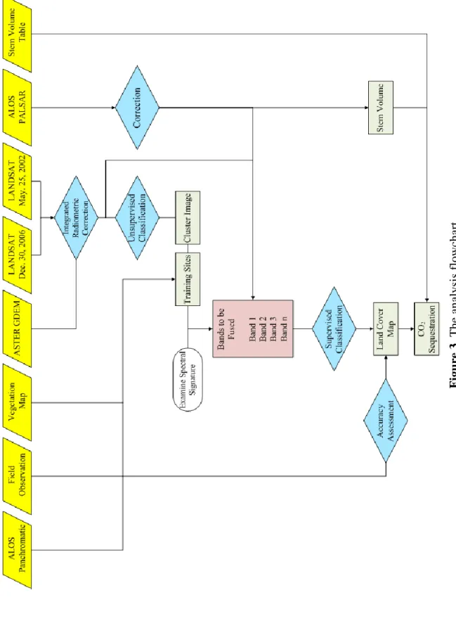
there. It could also simplify the process of monitoring of the environment. The overall flowchart of the methodology of this research is presented in Figure.3.

Figu re 3 . The a n alysi s flowc ha rt

(13)

7

3.1.1. GIS Software

In this research, the Clark Labs IDRISI Andes/IDRISI Taiga GIS platform was used for all the analysis. Various modules mounted and the high compatibility to other file format is the advantage of this software which will support our analysis. IDRISI Andes is the former version of IDRISI Taiga. Little changes in the interface and addition of new modules and supported file formats are the main differences although there are no minor changes in the calculations of the modules itself.

3.2. Gap Fill

As mentioned in section 2, the issue of the gap because of the SLC failure needs to overcome. Compared to the SLC-on data it can be seen that there are the gaps along the images on the SLC-off products (Figure.4 left). For the gap filling process, we used a frame and fill tool programmed by Richard Irish from NASA Goddard Space Flight Center. It uses the histogram matching method, calculating a transfer function which converts the radiometric values of one scene into equivalent radiometric values of a second scene, and then the transformed data are used to fill the gaps (USGS, 2004). After the gap filling process, the image can be seen with the gaps filled (Figure.4 right) and we assumed that this to be applicable for the analysis of the research.

(14)

8 Figu re 4 . The LAN D S AT ETM+ S LC -of f pr oduc t (D ec . 30, 2006) . P erf or manc e of the g ap fi ll , be for e ( on the l eft) a n d a fte r ( on th e r ight ).

(15)

9

3.3. Radiometric Correction

Performing radiometric correction (atmospheric and topographic) to the remote sensing images is a crucial issue especially when dealing with such analysis that depends strongly on the information of the electromagnetic spectrum of the earth’s objects. When the emitted or reflected electromagnetic energy is observed by a satellite sensor, the observed energy does not coincide with the energy emitted or reflected from the same object observed from a short distance. This is due to the solar azimuth and elevation, slope and aspects, atmospheric conditions such as haze or aerosols, etc. which influence the observed energy. Therefore, in order to obtain the actual irradiance or reflectance, those radiometric distortions must be corrected. For the correction of the images, we have applied the Integrated Radiometric Correction (IRC) method developed by Kobayashi & Sanga-Ngoie (2008). This method is a comprehensive radiometric calibration method aimed at simultaneous correction of atmospheric, solar, and topographic effects inherent to remote sensing data, which makes it possible to retrieve the at-surface reflectance and radiance values as if the atmosphere were totally transparent and the underlying surface was absolutely flat (Kobayashi & Sanga-Ngoie, 2008). The correction method follows with the atmospheric correction using the Dark Object Subtraction method and for the topographic correction, the derivation of solar and land geometric parameters, calculation of topographic correction factor, and atmospheric transmittance functions follows, then after retrieving these parameters we perform the IRC to fully correct the remote sensing imagery. The images were converted from Digital Numbers (DNs) to radiance values before entering the process.

Land geometric parameters can be derived from the DEM data. Using those parameters the cosine of the incidence angle (cosi) or the solar illumination and the h-factor which expresses the portion of the sky dome diffusing on to the tilted surface, can be given using equation (1) and (2):

Where, θz is the solar zenith angle, e is the slope angle between the inclined surface and the horizontal plane, Φe and Φs represents the aspect angle of the inclined surface from the north and the solar azimuth angle from the north respectively.

Topographic correction factor (A-factor) is then calculated with equation (3):

Where, C is the parameter calculated as the quotient between the regressional intercept and slope of the expression between cosi and surface radiance as sensed by the satellite. h0 is given by: (1) (2) (3) (4)

(16)

10

For the atmospheric transmittance functions, the Rayleigh scattering transmittance function (Tr) and water vapor transmittance function (Tw) was calculated. Expression (5) was used for the Rayleigh scattering transmittance (Trλ) as a function of wavelength (λ), the ambient atmospheric pressure (P) and the sea level atmospheric pressure (P0) in mbar.

Where M is the relative air mass expressed as:

For the atmospheric pressure (P) we did not assume P ≈ P0 as the author did since the elevation of the study area varied up to 1758 m at the highest, so instead we have used equation (7) to calculate the atmospheric pressure for each pixel locations.

Where, ai is the altitude at a certain pixel and a0 is the scale height. We have assumed the scale height to be 7900 m so that the model could match with the standard pressure described as a function of altitude by Holton (1992).

The water vapor transmittance function is a function of water vapor absorption coefficients (awλ), relative air mass (M) and precipitable water vapor (W) measured in centimeters. Given as:

For the precipitable water vapor, we could not get the spatial data so we have determined here

W to be a constant value.

With all the parameters calculated the expression for IRC yields finally:

Where, Lg is the corrected radiance from the surface, Ls* is the at-satellite observed spectral radiance from a sloped terrain and Lh is the upwelling atmospheric spectral radiance. All the optical data of 2002 and 2006 data from band 1 to 5 and band 7 was corrected through this process.

3.4. Vegetation Map

Producing a land cover map (detailed vegetation map) is one of the main objectives to achieve the goal for this research. The land cover map contains important information of what (urban, forest, water bodies etc.) is where and how much there are, and this map will be one of the source for the estimation of CO2 sequestration. The land cover map will be produced using the satellite remote sensing imagery. The year 2002 data will be the main data for the analysis

λ λ λ (5) (6) ₍₇₎ (8) (9)

(17)

11

while the year 2006 data and the PALSAR data will be a supplemental data for adding more information to the classification process for producing detailed land cover map.

3.4.1. Hybrid Classification

We have downloaded the polygon data of the administrative district published by the National and Regional Planning Bureau of Ministry of Land, Infrastructure, Transport and Tourism (MLIT). The polygon data of Oita prefecture is converted to a raster format Boolean image, and overlayed with the LANDSAT ETM+ image to extract the area of Oita Prefecture. All the bands from band 1 to band 7 (except band 6) are processed and for the PALSAR image too. The PALSAR image has been resampled to 30 m resolution using bilinear method to match with the LANDSAT imagery. The classification process for producing the land cover map will be based on this extracted imagery.

The Hybrid Classification method (Richards & Jia, 1999; Sanga-Ngoie & Kobayashi, 2003) is implemented for the classification process. This method uses both the unsupervised classification and supervised classification (Richards & Jia, 1999; Kato, 2004; Eastman, 2006), with the former classification first and on the base of the cluster image, which was produced by the unsupervised classification ISOCLUSTER module, the training site will be created and used in the supervised classification process. In the case of supervised classification, the software system delineates specific land cover types based on statistical characterization data drawn from known examples in the image (known as training sites). This “training sites” will be taken for each information classes (i.e. land cover types) and that information is then used to develop statistical characterization of reflectance/radiances for each information class as simple as the mean or the range of reflectance/radiances on each band, or as complex as detailed analyses of the mean, variances and covariances over all bands (Eastman, 2006). To verify the land cover type on the cluster image, the vegetation map published by the Ministry of Environment, Panchromatic data, and the information observed from the sites were utilized. The advantage of the hybrid classification is that when only supervised classification is implemented, its major drawback lies in the need to have delineated unimodal spectral classes beforehand, which by using unsupervised classification, this can be handled.

3.4.2. Maximum Likelihood

In the supervised classification, there are various methods for making decision about which pixel belongs to what classes. Parallelepiped, minimum distance to means, maximum likelihood, decision tree, linear discriminant analysis, etc. all of these methods differ only in the manner in which they develop and use statistical characterization of the training site data. In our analysis, the maximum likelihood method is used since this method estimates the posterior probability that a pixel belongs to each class, in other words, it gives the pixels to the most likely class based on the mean and variance/covariance data of the signatures from the training sites. This method is also the most widely used classifier in the classification of remotely sensed imagery. The spectral signature of each classes were examined through different bands to consider which bands will be used for the classification, while various

(18)

12

combinations of bands were experimented for checking which output gives the most reliable result. The images used for the classification is all radiometric corrected including the PALSAR data. The correction for the PALSAR data is described in section 3.6.2.2.

3.5. Accuracy Assessment

After the process of classification for producing land cover maps, accuracy assessment is an obligating process for evaluating the accuracy or the reliability of the map produced. The polygon data of the vegetation map published by the Ministry of Environment (Figure.5) was used assuming this as a ground truth, and the accuracy of the land cover map will be based on this information. Multiple sample points (over 29000) were generated using the stratified random sampling on the vegetation map to collect the ground truth points of the study area. Using this ground truth points and the land cover map, the accuracy will be assessed.

(19)

13 Figu re 5 . The ve g etation m ap (N ati ona l S ur ve y o n the N atura l Envi ronme nt) publi shed by the Mini stry of Environme nt . P art o f a r egion at t he study a re a.

(20)

14

3.5.1. Conventional Error Matrix

The ERRMAT module outputs the error matrix representing which classes matched the referenced classes, with the overall accuracy, omission and commission errors, and also outputs the information of Kappa Index of Agreement (KIA), and confidence interval. The Kappa value (K) can be calculated by equation (10)

Where P0 is the observed accuracy (proportion of agreeing units) and PC is the chance agreement (proportion of units for expected chance agreement). For the per-category Kappa (Ki) IDRISI follows the algorithm introduced to remote sensing by Rosenfield and Fitzpatrick-lins (1986):

Where Pii is the proportion of units agreeing in row i / column i and Pi+ is the proportion of units for expected chance agreement in row i, and P+i is the proportion of units for expected chance agreement in column i.

3.5.2. Fuzzy Accuracy Assessment - Fuzzy Error Matrix

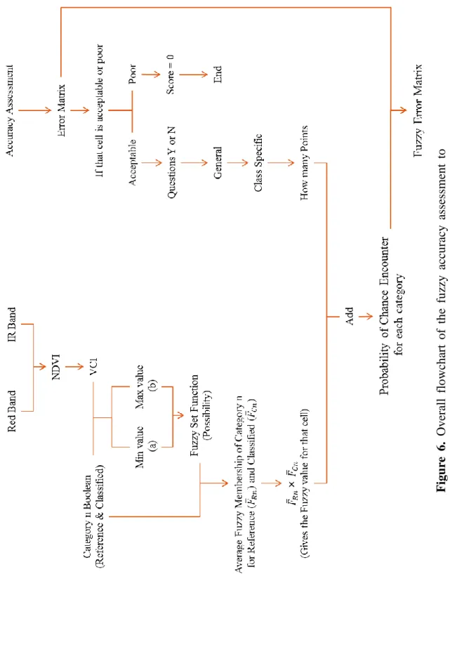
Fuzzy Accuracy Assessment is a concept that to focus more on the complexity of the environment and reflecting that in the accuracy assessment procedure. Gopal and Woodcock (1994) proposed the use of fuzzy sets to “allow for explicit recognition of the possibility that ambiguity might exist regarding the appropriate map label for some locations on the map. The situation of one category being exactly right and all other categories being equally and exactly wrong often does not exist.” It is recognized that instead of a simple system of correct and incorrect, there can be a variety of responses such as “absolutely right”, “good answer”, “acceptable”, “understandable but wrong”, and “absolutely wrong”. Green and Congalton (2004) introduced the technique called the fuzzy error matrix approach also stated by Congalton and Green (2009), which is a technique using the error matrix computed from the conventional accuracy assessment. It takes the process of generating a fuzzy error matrix from a set of fuzzy rules applied to the same classification that was used to generate the conventional error matrix. In the matrix it will not show just the correct or incorrect results, rather instead they will change this to accept or poor results. The categories which are in the category of accepted will be counted as a matched result while the poor will be considered as an error. Here we will implement this fuzzy accuracy assessment to reflect the reality (heterogeneity) of the environment in the accuracy assessment. The overall flowchart for this method is presented in Figure.6. (10) (11)

(21)

15 Figu re 6 . Ove ra ll flo wc ha rt of th e fu zz y ac cu ra cy assessment to modi fy the c onve nti ona l err or mat rix to t he f uz zy err or mat rix.

(22)

16

First, a set of questions (Table.1) are prepared for to answer which will be a weighting factor for the final assessment. The questions are based on the information of physical explanation or interpreters’ variability which could lead to an error of the land cover map. Each question is given weights so that according to the answer chosen, each category will be given that score. The questions will be answered for each cell in the matrix (the category where the reference and the classified class meets), although the cells to be answering the questions will be based on if that class is accepted to go through this procedure or not. If is considered as accepted, the procedure continues while if it is poor, that cell on the matrix will be ignored. The decision on if that cell is accepted or not depends on if the confusions between those classes could actually lead to the misclassification of the land cover (i.e. coniferous and evergreen forests), and if there is no way of getting misclassified it will be considered as poor (i.e. residential areas and water bodies).

(23)

17

G

en

er

al

Is

th

e

sa

te

lli

te

im

ag

e

co

rre

ct

ed

(a

tm

os

ph

eri

c/

to

po

gra

ph

ic

)

Y = 1 N = 0

Is

th

ere

a

li

m

ita

tio

n

in

th

e

re

fe

re

nc

e

da

ta

c

ol

le

ct

io

n

m

et

ho

d/

Is

th

e

re

fe

re

nc

e

da

ta

re

lia

bi

lit

y

un

ce

rt

ai

n

Y = 1 N = 0

Is

th

e

in

te

rp

re

te

r

va

ria

bi

lit

y

co

nt

ro

lle

d

Y = 0 N = 1

C

las

s S

pe

ci

fic

Is the s pe ct ra l s ign at ur e of the c la ss di ff ic ul t t o di ff er ent ia te w ith the m app ed cl as s Y = 2 Li ttl e di ff ic ul t = 1 N = 0

Is

th

e

cl

as

s

m

ore

d

om

in

an

t t

ha

n

th

e

m

ap

pe

d

cl

as

s

Y = 1 N = 0

D

oe

s

th

e

cl

as

s

ch

an

ge

it

s

sc

en

ery

in

a

nn

ua

l p

eri

od

o

f

tim

e

Y = 1 N = 0

Is

th

e

m

ap

pe

d

cl

as

s

ec

os

ys

te

m

h

ig

hl

y

he

te

ro

ge

ne

ou

s

Y = 2 T o some e xt ent = 1 N = 0

Sc

or

es

for

a

ns

w

er

T ab le 1. The que sti ons of the we ight ing fa ctors . T he que sti ons a re s epa ra te d int o two, o n e is the ge ne ra l and the oth er is the class spec ific. T he ge ne ra l ha s the ge ne ra l iss ue s whic h would lea d to an err o r as a ge ne ra l thi ng, while th e class spe cific will give s que sti ons that foc us on e ac h land f ea tur es.

(24)

18

Second, Vegetation Condition Index (VCI) (Kogan, 1998) will be used for the fuzzy set function computing the fuzzy membership (possibility) of each category. VCI can be calculated from the equation below:

Where, NDVIi is the NDVI value at a certain pixel, NDVImin is the minimum value of the NDVI and NDVImax is the maximum value of the NDVI. The Normalized Difference Vegetation Index (NDVI) can be calculated from the remote sensing imagery with the below equation:

Where, IR represents the infrared band of the satellite imagery and R for the red band imagery. NDVI is an indicator which can be used to analyze the activity of the vegetated areas. The value takes the range from -1 to 1 meaning that there are more activeness when the value becomes 1. This can be understood by the mechanism that the chlorophyll in the leaves has a character of reflecting the near infrared wavelength and absorbing more in the red wavelength, so by calculating this we can detect which area that has more greenness on the surface.

This possibility from the VCI will be added with the weighting factor from the questions and used for the calculation in the error matrix to decide the number of points (ground truth points) in each category, to be in the accepted or the poor.

3.6. Estimation of CO2 Sequestration

3.6.1. Estimation using Averaged Sequestration Value

Using the information of the total forest area derived from the land cover map, the estimation of the sequestration will be done by using the averaged sequestration values of each forest types observed by Tadaki and Hachiya (1968). Multiplying the total forest area by the averaged value per unit area will give us the results of the total sequestration value of each forest types. The sequestration value is the aboveground Net Primary Product (NPP), which is the value of the CO2 absorbed from the photosynthesis process subtracting the respiration activity (Matsumoto, 2001).

3.6.2. Estimation Considering Tree Age

Not only with the simple estimation for each forest types, but the estimation considering tree ages were examined. This is due to the differences in the sequestration rate among different tree ages, so by considering the sequestration per tree age, it would be a more precise estimation rather than using only the averaged sequestration value. Therefore we have estimated the tree ages based on two methods, one is using the optical data computing NDVI and using that to classify the ages of the forests, and second is using the microwave data to classify the forest area into tree ages categories.

(12)

(25)

19

3.6.2.1. Classifying Tree Age based on NDVI

The relationship between NDVI and tree age was deduced by Ishii (2007) based on the Forest Tree Age growth curve and multi-temporal NDVI data (Figure.7).

Figure 7. Forest Tree Age growth curves (Ishii, 2007). Different forest types in multiple locations from Vietnam, Thailand and Japan. The blue line shows the Japanese Sugi (Cedar) Forests growth curve.

Referring to this growth curve, we could thus classify the coniferous forests area into separate tree ages categories. The classification of the tree ages was implemented only to the coniferous (cedar) forests by using this method, since the relation between the NDVI and forest tree age growth was analyzed with that type of forests.

3.6.2.2. Classifying Tree Age based on Stem Volume

The PALSAR data was used for the analysis of stem volume, so that the tree ages can be known. The DN values were converted to the backscattering intensity (σ0) in decibel units using equation (12)

CF is the calibration factor for the PALSAR product, for the level 1.5 product CF=-83.0 dB. For a correct interpretation of the backscatter signatures, corrections for the effect of local incidence angle and normalization for the true pixel area were necessary.

The corrected backscatter in gamma nought (γ0) format can be obtained from the sigma nought (σ0) value according to Castel et.al (2001) and Ulander (1996), which has also been applied by other authors (Chen et.al, 2009; Santoro et.al, 2009; Armston et.al, 2010; Santoro et.al, 2011).

(26)

20

Where, θloc and θref represents the local incidence angle and a reference angle for the normalization of the backscatter (e.g. off nadir angle) respectively. Aslope and Aflat represents the true pixel area and the local pixel area for a theoretically flat terrain respectively. For details refer to Castel et.al (2001) and Ulander (1996). For bare surfaces, the exponent n is equal to one. For vegetated surfaces, it expresses the variation of the scattering mechanism due to the presence of a volume on the sloped terrain, thus being related to the optical depth of the vegetation. At the forest site of Lozere, France, the value was estimated lower and equal to 0.36 for the Japanese Earth Resources Satellite (JERS)-1 L-band SAR backscatter. The lack of detailed information about optical depth of the forest canopies at the study area was determined but we have applied the 0.36 value since that the scattering properties of the forests should be taken into account. For future works, this should be reconsidered for the case of different polarizations also. In the case of γ0, as opposed to the case of σ0 or β0, the unit area is taken perpendicular to the axis of the radar beam.

The relationship between backscattering intensity and stem volume or biomass has been analyzed by various researchers (Kuplich et.al, 2000; Champion et.al. 2008; Karjalainen et.al 2008; Chen et.al, 2009; Wijaya, 2009; Santoro et.al, 2011). Through various studies, it is stated that the backscattering signature correlates with the forest parameters, and it has been shown in many studies that SAR images can be used to extract forest biomass related information. Because of time, we did not have a chance of collecting ground data of the stem volume in our study area, so we have implemented the polynomial model developed by Wijaya (2009) (equation (14)) to estimate the stem volume.

Where, V is the stem volume and σ is the backscattering intensity. The reason we used this model was because the data they have used was the most similar data compared to our data (PALSAR L-band FBD 34.3˚ HH/HV specifications). The stem volume map produced using this model was then classified into ages among the forests referring to the relationship of the tree age and stem volume information provided by Oita Prefectural Government. The classification was done to the coniferous and deciduous broad leaf forests but not the evergreen broad leaf forests because there were no data for that forest type. The data of Sugi (Cedar) and Saw Tooth Oak was used as the coniferous forests and deciduous broad leaf forests respectively.

4. Results

4.1. Evaluation of Radiometric Correction

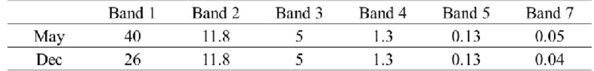
Before performing the IRC, the remote sensing images were needed to be corrected for atmospheric effects. The Dark Object Subtraction method was implemented and the radiance value was computed for all the bands for correction (Table.2) and as you can see the

(15)

(27)

21

remarkable decrease in the haze value with the increasing of wavelengths. This haze value was subtracted by the whole pixel values on the image.

Table 2. Computed haze values: Lh (measured in Wm-2 μm-1 sr-1).

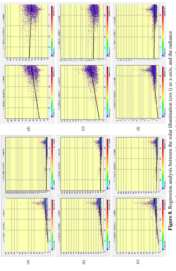
After the atmospheric correction, the IRC is performed. Quantitative evaluation of the

performance of the correction is done by assessing the non-correlationship between the solar

illumination (cosi) and the corrected data. In Figure.8, it shows the regression analysis between the solar illumination and non-corrected data on the left, which can be seen with a high correlation, with higher radiance for higher cosi value because of topographic effects. However, in the same Figure.8 on the right, the correlation between those two can be seen with lower or mostly non correlation which is the data after the correction. Figure.9 shows the example of the difference of images before the correction and after for band 4. The zoomed area is a mountainous location and the radiance values are corrected in those areas, while the areas on the top left side can be seen without the changes where it is the residential areas.

(28)

22 Figu re 8 . R egr essi on a na lysi s betw ee n the solar il lumi na ti on (c os i ) as x -a xi s, and the ra dian ce va lue a s y -a xis for ( a) ba nd 1 ( b) ba nd 2( c) ba nd 3 (d) ba nd 4( e) ba nd 5 and (f ) ba nd 7 .

(29)

23 Figu re 9 . Or igi na l ne ar -infr ar ed ba nd (b and 4) im age (le ft) a nd IRC cor re ct ed im age ( right) in r adianc e ove r the st udy a re a.

(30)

24

4.2. Land Cover Map - Vegetation Map 4.2.1. Extracting Oita Prefecture

Using the polygon data of the administrative district, it has been overlayed with the LANDSAT and PALSAR images for each bands and polarization to extract the study area (Figure.10). This area will be the area for the analysis and the images will be the bases for the analysis of unsupervised and supervised classification.

Figure 10. Extraction of Oita Prefecture for LANDSAT ETM+ (a) band 1 (b) band 2 (c) band 3 (d) band 4 (e) band 5 (f) band 7 and PALSAR (g) HH (h) HV.

4.2.2. Unsupervised Classification

Using the images which the study area was extracted, the unsupervised classification ISOCLUSTER module was performed to produce a cluster image (Figure.11). Corrected images band 1 to 5 and NDVI data was used with 100 times iterations outputting 20 classes.

(31)

25

On this image, you can see the cluster of each classes but not identified as what land cover it is corresponding to. The training sites will be constructed on the top of this cluster image so it can be handled easier for where the class border changes. The constructed training sites will be used in the latter supervised classification process.

Figure 11. Cluster image produced by the ISOCLUSTER module.

4.2.3. Supervised Classification

Comparing with the supervised classification alone, the process of constructing the training sites are more accurate and it will result with higher accuracy of the land cover map due to the precise information of the spectral signature of that certain land cover type.

Figure.12 shows the spectral signature of each land cover types along different bands of LANDSAT ETM+. The y-axis is the radiance unit and the values for each class are represented with the mean radiance of the pixels taken by the training sites. Similarity can be seen among some classes (e.g. forests) although totally different spectral signature can be seen in some other classes (e.g. residential area and water bodies). This spectral difference is the characteristics of those classes for to differentiate with other classes.

(32)

26

Figure 12. Signature comparison between land cover types. It is the mean radiance value taken from the pixels where the training sites were constructed. 1 to 7 is the May data mean value from band 1 to 7, while w1 to w7 is the December data mean value from band 1 to 7.

4.2.4. Maximum Likelihood

MAXLIKE module uses the spectral signature of the classes with the images to be fused, and the pixels will be classed to the most likely classes they would belong according to the algorithm. The final product of the land cover map is shown in Figure.13 which is the reclassified map from the original 12 classes to 10 classes. The category of 12 classes and the 10 classes are shown on Table.3 with which class was merged to what class. This product was chosen from the various outputs made by using various bands of satellite images to see the differences of accuracies among them all shown on Table.4. May and Dec represents which month data sets were used in the process, while NDVIMay is the NDVI data from the May data and NDVIDec is the data from December. HV is the PALSAR HV polarized backscattering data and the correct and no correct is if the images were radiometric corrected or not.

(33)

27 Figu re 1 3 . The f inal out put of the la nd c ove r ma p .

(34)

28

Table 3. Land cover classes. Left = Original output; Right = Final product.

Table 4. Accuracy of the land cover map from the classification process, on the combination of multiple images with Type A = 12 class and Type B = 10 class.

4.3. Accuracy Assessment

4.3.1 Conventional Error Matrix

The ground truth points obtained from the reference data was used with the land cover map to perform the accuracy assessment by outputting the error matrix (Table.5).

(35)

29 T ab le 5 . Er ror Matr ix sh owing the r ef ere n ce da ta ve

rsus the image

c la ssi fic ati on . R efe re nc e C o n if er o u s Sil v er Gr ass Gr ass lan d s B ar e lan d s W ater b o d ies C ro p lan d s P ad d y f ield s R esid en tial Dec id u o u s-Bl E v er g ree n -Bl T o tal E rr o rC User s A C o n if er o u s 9305 100 52 16 61 125 158 39 1086 1543 12485 2 5 .4 7 % 7 4 .5 3 % Sil v er Gr ass 6 365 48 7 2 7 3 1 17 0 456 1 9 .9 6 % 8 0 .0 4 % Gr ass lan d s 69 192 211 17 8 86 71 26 65 18 763 7 2 .3 5 % 2 7 .6 5 % Classifie d B ar e lan d s 5 10 14 41 12 5 7 59 3 2 158 7 4 .0 5 % 2 5 .9 5 % W ater b o d ies 5 9 2 12 279 0 8 6 1 14 336 1 6 .9 6 % 8 3 .0 4 % C ro p lan d s 179 29 67 52 28 235 237 197 42 71 1137 7 9 .3 3 % 2 0 .6 7 % P ad d y f ield s 309 128 129 109 223 216 1339 349 120 105 3027 5 5 .7 6 % 4 4 .2 4 % R esid en tial 5 15 40 55 70 34 104 651 7 9 990 3 4 .2 4 % 6 5 .7 6 % Dec id u o u s-Bl 1190 363 129 18 4 85 73 12 1788 500 4162 5 7 .0 4 % 4 2 .9 6 % E v er g ree n -Bl 1734 77 89 25 16 257 108 44 1123 1729 5202 6 6 .7 6 % 3 3 .2 4 % T o tal 12807 1288 781 352 703 1050 2108 1384 4252 3991 28716 Er ro rO 2 7 .3 4 % 7 1 .6 6 % 7 2 .9 5 % 8 8 .3 5 % 6 0 .3 1 % 7 7 .6 2 % 3 6 .4 8 % 5 2 .9 1 % 5 7 .9 5 % 5 6 .6 8 % 4 4 .4 8 % Ov er all A ccu rac y P ro d u ce rs A 7 2 .6 6 % 2 8 .3 4 % 2 7 .0 2 % 1 1 .6 5 % 3 9 .6 9 % 2 2 .3 8 % 6 3 .5 2 % 4 7 .0 4 % 4 2 .0 5 % 4 3 .3 2 % 1 5 9 4 3 /2 8 7 1 6 = 5 5 .5 2 %

(36)

30

Here, the reference data (ground truth) is presented in the column and the classified category is in the row. Major diagonal of the error matrix represents agreement between the reference data and the classified map, and is represented by a single cell in the matrix for each map class. It is computed with the user’s accuracy (Error of Commission) for the row total and the producer’s accuracy (Error of Omission) for the column total. The overall accuracy is considered with sum of the points which has the exact match between the reference data and the classified data (major diagonal in bold) divided by the total number of points. The overall accuracy of the land cover map resulted at 55.5 % which was produced using the May and December data with the NDVI data of both months.

4.3.2. Fuzzy Error Matrix

Now on the base of this error matrix, the fuzzy error matrix is developed. But, to consider how many points that will be considered as the accepted or poor will be determined by the method developed here. Table.6 shows the total scores for each category based on the set of questions from Table.1.

Table 6. The scores per category for the accepted classes from the questions.

The VCI is calculated by the NDVI and it will be used in the process for computing the degree of possibility for each category by using the fuzzy set membership function. The minimum and the maximum value of the VCI are checked for each land cover classes of the classified data and the reference data. Each minimum and the maximum VCI values are used as the inflection points for the sigmoidal membership function as the start point and the end point. The sigmoidal decreasing function is used for the bare land, water body and residential classes, and sigmoidal increasing function is used for the rest of the classes (Figure.14). The averaged possibility value is then computed from the obtained fuzzy membership.

(37)

31

Classified VCI Min (a)

Classified VCI Max (b)

Reference VCI Min (a)

Reference VCI Max (b)

Average Fuzzy Value (Classified)

Average Fuzzy Value (Reference) VCImean Fuzzymean VCImean Fuzzymean

Coniferous 0.410134 0.96572 0.301876 0.977906 0.884192 0.948527 0.888412 0.94567 Silver Grass 0.560172 0.952448 0.265581 0.950968 0.829053 0.828093 0.852293 0.893879 Grasslands 0.390919 0.99717 0.295296 0.99717 0.76913 0.70294 0.779216 0.738551 Bare lands 0.0635 0.944625 0.111345 0.943727 0.655491 0.560937 0.469618 0.304187 Water bodies 0.048604 1 0.000002 0.940239 0.590886 0.533819 0.502571 0.333754 Crop lands 0.362285 0.944637 0.396596 0.952158 0.772072 0.619373 0.701587 0.722922 Paddy fields 0.000002 0.948069 0.244144 0.948178 0.673445 0.781971 0.663452 0.646427 Residential 0.222579 0.940738 0.153129 0.950462 0.618035 0.567961 0.548372 0.38621 Deciduous-Bl 0.707479 0.966771 0.353214 0.966771 0.901192 0.896936 0.916275 0.96095 Evergreen-Bl 0.446955 0.977906 0.308070 0.960948 0.892351 0.934219 0.89359 0.954593

Figure 14. The sigmoidal membership function produced using a cosine function. The points a to d (along the x-axis) represents the inflection points governing the shape of the curve for (a) monotonically increasing shape and (b) monotonically decreasing shape.

The minimum VCI value and the maximum value used for each class as the inflection points, average degree of possibility for each land cover classes of the classified data and the reference data is listed in Table.7 and the average possibility values for each category were calculated by multiplying with the reference category and the classified category value to fit into the matrix (Table.8).

Table 7. List of the VCI value used in the fuzzy membership function, and the average fuzzy value computed for each of the classes of the classified map and the reference map.

(38)

32 Reference

Coniferous Silver Grass Grasslands Bare lands Water bodies Crop lands Paddy fields Residential Deciduous-Bl Evergreen-Bl

Coniferous - 0.9115 0.9055 Silver Grass - 0.5821 0.5986 Grasslands 0.6283 - 0.5082 0.4544 Bare lands - 0.3626 0.2166 Water bodies - 0.3451 Crop lands 0.5536 0.4574 - 0.4004 0.2392 Paddy fields 0.699 0.5775 0.2379 0.261 0.5653 - 0.302 Residential 0.1728 0.4106 0.3671 -Deciduous-Bl 0.8482 - 0.8562 Evergreen-Bl 0.8835 0.8977 -C lass ified

Table 8. Each value represents the fuzzy value computed from the VCI for the accepted category given by: Average Fuzzy Value (Reference) × Average Fuzzy Value (Classified).

The value in the matrix is computed from calculating the mean fuzzy value of each category for the reference and the classified category and multiplying them together. This will be added with the score obtained from the questions generating a final score which will show the percentage of how many points should be considered as accepted, while the rest will be considered as poor (Table.9).

Table 9. The Probability of Chance Encounter (%) is computed to each of the categories which were accepted, by adding the scores from the questions and the value from the fuzzy set function. The percentages of the sample points in that category will be counted for the overall accuracy and for both producers and users accuracy.

The final output of the fuzzy error matrix is shown in Table.10 where the matrix is modified by separating the non-diagonal cells into accept and poor, and the points that belongs to “accept” are considered to be a “match” for estimating fuzzy accuracy. Fuzzy overall accuracy has resulted 79.3 % for the same land cover map which the accuracy was assessed in the conventional error matrix (55.5 %). This method is an alternative way of considering the accepted and poor, in the situation of if the accuracy assessment is based on a third party reference data and not by the primary ground data which has been collected at site. This method implies the consideration of the misclassification caused by the known physical explanation and the interpreter’s variability by weighting them. While it also considers the issue of the appropriateness of the sample unit, especially the problems stated when using the single pixel as the sample unit (Congalton and Green, 2009).

(39)

33 T ab le 10 . F uz zy Er ror M atrix following t he s ame methodology as tra dit ion al er ro r ma trix with t he following addit ions: Non -diagona l ce ll s in the matrix contains ac ce pte d and poor . W hil e the number s in the ac ce pted are c onsi de re d a “matc h ” for e sti mating fuz zy ac cur ac y, the number s in the poor wa s consi de re d as an err or . T he fu zz y ov era ll a cc u ra cy is esti mate d as the pe rc entag e of sit es whe re the ac ce ptabl e r ef ere n ce lab els m atche d the c lassifie d labe l.

(40)

34

4.4. CO2 Sequestration by Forests in Oita Prefecture

Referring to the observation by Tadaki & hachiya (1968), CO2 sequestration by each forest types were calculated (Table.11). It has resulted total sequestration of coniferous forests at; 3.56 MtCO2/yr, deciduous broad leaf forests; 0.77 MtCO2/yr, and evergreen broad leaf forests; 2.25 MtCO2/yr, totaling 6.59 MtCO2/yr for all the forest cover together.

Table 11. CO2 sequestration by each forest types of the study area.

4.5. CO2 Sequestration by Forests in Oita Prefecture per Tree Age

4.5.1. Sequestration per Tree Age based on NDVI

For a deeper consideration of estimation of the coniferous forests, it was classified into per tree ages using the NDVI. On the left of Figure.15, shows the NDVI image for the study area. This is then reclassed into an image where each class representing ranges of the NDVI value (Figure.15 on the right). Each value range represents which age the coniferous tree would be according to Ishii (2007).

(41)

35 Figu re 1 5 . O rigina l ND VI im age o f the study a re a on th e lef t, and the re classe d ND VI im age on th e r ight . T he ra ng e of N D VI is c ompatibl e with t he S ugi t re e a g es.

(42)

36

This reclassed NDVI image is overlayed with the boolean image of a coniferous area so that the coniferous area for per tree ages can be extracted. As shown in Table.12, the tree age was classified into 4 ranges and the sequestrations per ages were calculated from the CO2 sequestration table published by Tochigi Prefectural Government (2010). The total sequestration of the coniferous forests has resulted 2.35 MtCO2/yr, comparing with when the averaged value was used for per forest type, the resulting value has decrease more than 34 %. However, when we see the sequestration value for per tree ages, the value shown in the 10-15 year coniferous trees are the ones that sequestrate CO2 the most among other ages and contributing to the concept of carbon sink. It is also very similar to what was applied for the per forest type value, meaning that the averaged value used for per forest types can be a problem for overestimating the forests potential capacity and it is not good when we need a precise estimation for the carbon capacity.

Table 12. CO2 sequestration of the Sugi-Hinoki forest area per tree ages.

4.5.2. Sequestration per Tree Age based on Stem Volume

The stem volume map was produced using the backscattering intensity derived from the PALSAR data (Figure.16). Regarding to the stem volume table provided from the Oita Prefectural Government (modified and shown as a graph on Figure.17), the stem volume map was reclassed to the ranges of stem volume which will represent the range of ages. The range of the stem volume was reclassed considering the different growth rate among the regions of the study area. We found that in the Hita region, on the western region of Oita Prefecture, the coniferous forests in the age of 15-20 is more distributed among this area, while the age over 20 is distributed all along the Prefecture except for the Hita region. This could be understood by the features of Hita region, because they implement continuous afforestation activities and is very famous for forestry (wood products, etc.). However, in the other regions of Oita, the forests are left without any treatment so it shows older ages of the forests. For the deciduous forests, it is mostly a natural forest, so the distribution of the forests is mainly in the years over 30 (it is left naturally without human activity) and distributed all around Oita Prefecture.

(43)

37

(44)

38

Figure 17. Stem volume as a function of tree age. The Sugi (Cedar) tree age curve on the top and Saw Tooth Oak on the bottom (Oita Prefecture). The growth of stem volume varies among different regions of the study area.

立命館学術成果リポジトリ

Estimating CO

Sequestration by Forests in Oita Prefecture, Japan,

Combining LANDSAT ETM+ and ALOS Satellite Remote Sensing Data

Kotaro Iizuka

(Student Number 51210012)

January 2012

Table of Contents

List of Figures

List of Tables

Abstract

要約

G

en

er

al

Is

th

e

sa

te

lli

te

im

ag

e

co

rre

ct

ed

(a

tm

os

ph

eri

c/

to

po

gra

ph

ic

)

Is

th

ere

a

li

m

ita

tio

n

in

th

e

re

fe

re

nc

e

da

ta

c

ol

le

ct

io

n

m

et

ho

d/

Is

th

e

re

fe

re

nc

e

da