Title
スロットを用いた環状型ネットワークにおけるフルロー
ド・トラヒックの解析
Author(s)
照屋, 健; 白鳥, 則郎
Citation
沖縄大学マルチメディア教育研究センター紀要 = The
Bulletin of Multimedia Education and Research Center,
University of Okinawa(5): 31-38
Issue Date
2005-03-31
URL
http://hdl.handle.net/20.500.12001/6403
ス ロ ッ トを用 いた環状型ネ ッ トワー クにお ける
フル ロー ド ∴トラヒックの解析
照
崖
健
I白
鳥
則
郎 I
I
I沖縄大学
法経学部
教授
I
I東 北 大 学
電気通信研究所
教授
あらまし 一般 に、ネ ッ トワー ク ・トラヒックの混雑 は大別 して三つの状態 に分類 され る。いわゆる軽 い負荷、中 程度の負荷、重い負荷の三つの状態である。 フル ロー ド状態のシステムを研究す ることは重 い負荷の状態 におけるシステムの動作 を予測す るのに極 めて有用 で ある。【
3
日4
】
本稿で は、 フル ロー ド状態のシステムにおけるパケ ッ ト伝送の過渡状態 を解析 し、そのネ ッ トワー クの トラヒック 特性 を導 出す る。Ana
l
ys
ュ
●
sO
nFul
l
-
Loa
d
T
r
a
f
Bci
naSl
o
t
t
e
dRi
ngNe
t
wo
r
k
Ke
nTERUYAIa
ndNo
r
i
oSHI
RATORI
I
I
tPr
of
e
s
s
or
,
Fac
ul
t
yofLa
w andEc
onomi
c
s
,
Oki
na
waUni
ve
r
s
i
t
y
H Pr
of
e
s
s
or
,
R.I
.
E.
C.
,
TohokuUni
ve
r
s
i
t
y
Abs
t
r
ac
t l
nge
ne
r
a
l
,
t
r
a
f
Rcc
on
J
●
e
S
t
i
onofane
t
wo
r
ka
r
ec
l
a
s
s
i
f
ie
di
nt
ot
hr
e
ec
a
t
e
g
or
i
e
s
,
na
me
l
yl
i
g
ht
l
y
l
oa
de
d
,
i
n
t
e
r
me
di
a
t
e
l
yl
oa
de
da
ndhe
a
vi
l
yl
oa
de
dc
o
ndi
t
i
ons
.
Tos
t
udyo
ft
hes
ys
t
e
munde
rf
ul
ll
oa
dc
ondi
t
i
o
ni
sus
e
f
ulf
ors
pe
c
ul
a
t
i
ngt
hebe
ha
v
io
ro
ft
hes
ys
t
e
mi
nhe
a
v
il
y
l
oa
de
dt
r
a
氏cc
ondi
t
i
ons
l
3
日4
]
・
I
nt
hi
spa
pe
r
,
Wea
na
l
yz
et
het
r
a
ns
i
e
nts
t
a
t
eofpa
c
k
e
tt
r
a
ns
mi
s
s
i
ona
ndde
r
i
vet
r
a
f
Rcc
ha
r
a
c
t
e
r
i
s
t
i
c
so
ft
he
ne
t
wor
k.
1.
Introduction
There are broadly two categories of ring network, namely the token-ring type and the slotted ring type. The former is often used for LAN networks and the latter is utilized for control systems.
In this paper, we focus on the slotted ring, and derive transient state characteristics of the informa tion transmission rate.
In the past, we have reported [1][3] certain characteristics of slotted ring networks. However, results are mainly discussed in terms of average values such as average queue length or average waiting time, and the transient characteristics are left mostly unsolved due to the difficulty of analysis.
In this paper, we derive transient characteristics of the information transmission rate in the cases of rings of three and four stations.
2.
Definitions and model description
2.1 Definitions
[Definition 1] (Address distribution probability.) Let the address distribution probability d{ be the
probability that the destination of a packet generated at a certain station is the i - th (1 £ i ^ TV - 1) station in the direction of transmission, taking the originating station as zero. Thus the equation
X^i* di = 1 is satisfied, where N is the number of stations connected to the ring.
[Definition 2] (State of slot.) The address of the packet which is mounted on the slot departing from station Si in Figure 1 is assumed to be that of one of the other stations, i.e. Si+i, $+2? • • • ? Si+j , • • • , or Si+N-i, we then define the state of the slot to be A\, A^ • • • , Aj , • • • , or An-u respectively.
Here, i + N — 1 is congruent to i — 1, modulo N.
[Definition 3] (Slot state transition.) Each passage of the slot past successive stations marks the
completion of one step in the cycle of slot around the ring, and is assumed to require a fixed time. As
the state of the slot changes with each passage, this passage is also referred to as a slot state transition.
[Definition 4] (Slot state probability vector.) Let Xi(n) be the probability that the n-th slot state
transition is to the state Ai. Then the vector X(n) which has components Xi(n), i — 1, • • •, N - 1, is defined as the slot state probability vector, i.e.
X(n) =
[X1(n),X2(n)r-where Xx{0) = 1, and X;(0) = 0
for (2£i£N-l).
The initial conditions for n = 0 imply that a vacant slot is incoming to station Si, i.e. the initial slot
is A\.
[Definition 5] (Information transmission rate.) The information transmission rate of the system is defined as the average number of packets that flow out of a station per unit time. The transient information transmission rate is defined as the number of packets that flow out of a station per step.
symbolize it with Ajy(n), (N = 3,4, • • •), where N and n denote number of both stations and transitions respectively. Here, we consider that N = 3 is the minimum number of the station to form the ring.
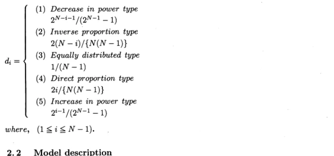
[Definition 6] (Pattern of address distribution probability.) The following patterns are introduced
as examples of address distribution probability. (1) Decrease in power type (2) Inverse proportion type (3) Equally distributed type
1/(N-1)
(4) Direct proportion type (5) Increase in power type
where, (1 £ i ^ N - 1).
2. 2 Model description
Figure 1 shows the slotted ring network considered in this study and Fig.2 shows the model of a station in the ring. We first consider general system of N stations forming a ring. The analysis
Fig.l Model of a network
Direction of TYansmission Writing Ring line Reading (Terminal)
Fig.2 Model of each station
is based on the following assumptions: (a) The packets are of fixed length equal to the slot length, (b) packets are waiting under full load conditions in each station, (c) the transmission of the packet
on the ring is unidirectional and clockwise as shown in Figure 1, (d) packets generated at any origin station are accurately and reliably detected, received and eliminated at their respective destination
station, and (e) address distribution probabilities at every station are identical.
In general, traffic conditions of a network are classified into three categories, namely lightly loaded, intermediately loaded and heavily loaded conditions. To study of the system under full load condition is useful for speculating the behavior of the system in heavily loaded traffic conditions.
It will be helpful for clarifying the characteristics of the system studying such matters as the cal culation of the maximum value of information transmission rate and investigation of the relationship
between maximum value of information transmission rate and address distribution probability. Fur thermore, we can tell that the transient analysis is the useful means to research on the details of the
system behavior which varies at every slot transitions.
We consider the transition probabilities pij that a slot in state Ai undergoes a transition to state
j. These are given as follows [3]: 1, j = i-0, j
where i, j = 1, 2, • • •, N — 1. The transition probabilities can be expressed in matrix notation
by placing transition probabilities pij in the (i,j) location. Here, di denotes address distribution
probability ( Definition 1). h 1 0 0 1 dz ... 0 ... 0 ... "JV-l 0 0
(2)
3.
Transient characteristics of information transmission rate
3.1 Power of transition probability matrix
[Lemma 1] In the case of N = 3, if patterns of address distribution probability as those defined in definition 6, the n-th power of the transition probability matrix which is generated after n transitions
is given as follows:
3 = d2
d2
[Lemma 2] In the case of N = 4, if patterns of address distribution probability as those defined in definition 6, which satisfy D(= (1 - di)2 - 4d3) < 0 , the n-th power of transition probability matrix,
P41, which is generated after n transitions is given as follows:
A — T"
r{u)\
-r((jj\ - UJ2)
— r2u>2)r2u2 —ru;2(l — —ru;2(l — A
— (1 — r2u)2)r2u2
—(1 — 22
—(1 — r2uj2) - ruji) where A = (A2 - A3){A2A3 - (A2 + A3) + 1}= ^(^i ~~ ^2)(2 ~~ d\ + d3),
uj\ = exp(i9), 0J2 = exp(—i0), r = y/ds, O = ir — (1 d{)2)/{I -[Lemma 3] In the case of N = 4, for patterns of address distribution probability other than those defined in definition 6, which satisfy D > 0, n-th power of the transition probability matrix is given as follows: -r2(l - r2)r\ -r2(l-r2)ri •pn _ ■*■ A n-r2 ~{r{-r$) ri _ r2 —{r2 — r!)
(1 — r\)r\ —(1 — T\)t\
(i-ri)
-(l-r?)
nil-n)
-r2(l-r2) where r\ = „—— + — di)2 — 4d3 T2 = 2 2 2A = (7*1 - r2){l - (ri + r2) + rir2} = (ri - r2)(2 - d\ + d3).
[Lemma 4] In the case of N = 4, for patterns of address distribution probability other than those denned in definition 6, which satisfy D = 0, n-th power of the transition probability matrix is given as follows: n _ 4 1 1 0 1 -1 1 (l-di)/d3 1 0 0 0 n rn u r0 0 0 (1 - di + where A = 2 — di + d -(1 - di) l-d3 (l-di+d3)/d3 2d3)/2
3. 2 Transient characteristics of the information transmission rate
[Theorem 1] In the case of N = 3, if patterns of address distribution probability are given by definition 6, the transient information transmission rate for n transitions is given by :
As(n) = !±£=^
[Theorem 2] In the case of N = 4, if patterns of address distribution probability are given by definition
6, which satisfy D < 0, the transient information transmission rate for n transitions is given by :1
A4(n) =1
2-d1+d3 ()/ {l-rn+1
+ 2 J2 cos(2(k + 1)0))
k=Q +2rn+2 J2 COs(2k+l)9)} k=0 ; for odd n n/2 fe=0 +rn+2(l+2 ; for even n (n-2)/2 k=0[Theorem 3] In the case of N = 4, for patterns of address distribution probability other than those defined in definition 6, which satisfy D > 0, the transient information transmission rate is given as
follows:
[Theorem 4] In the case of N = 4, for patterns of address distribution probability other than those
defined in definition 6, which satisfy D = 0, the transient information transmission rate is given asfollows: A4(n) =
where r0 = -(1 - di)/2.
3. 3 Numerical Examples
Characteristics of the transient information transmission rate are shown in Figures 3, 4 and 5 for the case of three and four stations connected to the ring respectively.
The abscissa denotes the number of transitions n and the ordinate denotes the normalized transient information transmission rate Ajv(n).
These figures show that the transient information transmission rate attains steady-state in the
period between approximately 5 and 12 transitions.
A lower transient information transmission rate is achieved after a larger number of transitions for the case of the proportionally increasing pattern of address distribution probability, compared to
results for the equal address distribution probability.
The converse is true for the inversely proportional pattern considered; a steady higher rate is
achieved in a lower number of transitions.
▲ — : Inverse proportion
■ — : Equally distributed
# — : Direct proportion
0 5 10
77, (transitions) Fig.3 Transient information transmission
rate (N=3) 1 -0 0 A A -— ■ — • O -v M fl -^ : Decrease in power : Inverse proportion : Equally distributed : Direct proportion : Increase in power ■ ■ ■ i ■ 5 10 77, (transitions) Fig.4 Transient information transmission
rate (N=4)
The limiting values of the transient information transmission rate agree well with the steady-state val ues reported previously[3]. Our results also reflect the tendency for the magnitude of the steady-state transient information transmission rate to decrease as the number of stations connected to the ring
1F
0.5 A — : Special case # 1 8/16 : 7/16 : 1/16 O - : Special case # 2 1/9 : 7/9 : 1/9 _l . , , . I . . . . l_ 0 5 10 71 (transitions)Fig.5 Transient information transmission rate (N=4)
This type of network involves the interaction of traffic between stations. The results of this study suggest that the pattern of communication traffic between stations must be taken into consideration
when designing the network topology.
4.
Conclusions
In this paper, we have discussed the transient characteristics of the system throughput in a slotted ring network and have reported several expressions for them. Our next goal is the derivation of general formulas for these transient characteristics.
References
[1] N. Shiratori, S. Noguchi and J. Oizumi, "On buffering in computer networks," Trans. D, vol. J59-D,
no.6, pp.398-405, June 1976.
[2] W. W. Chu, "Buffer behavior for Poisson arrivals and multiple synchronous constant outputs," IEEE,
Trans. Commun., vol. COM-19, no.6, pp.530-534, June 1970.
[3] K. Teruya, N. Shiratori and S. Noguchi, "A performance evaluation method of a slotted loop network,"
IEICE Trans. A, vol. J70-A, no.2, pp.289-300, Feb. 1987.
[4] K. Teruya and N. Shiratori, "Evaluation of transmission control method in a slotted ring network,"
IEICE Trans. A, vol. E78-A, no.ll, pp.1519-1526, Nov. 1995.
[5] W. Bux, "Local-area subnetworks: a performance comparison", IEEE Trans. Commun., vol. COM-29,