The Effect of Reversible Investment on Credit Risk (Financial Modeling and Analysis)

(1)

The Effect of Reversible

Investment on

Credit Risk1

大阪大学経済学研究科全海濬 (Haejun Jeon)

Graduate SchoolofEconomics

Osaka University

大阪大学・経済学研究科西原理(Michi Nishihara)

Graduate School of Economics

Osaka University

1 Introduction

A firm’s decision to invest isoneof the most important issues in finance. Recently, a real option

basedapproachissowidelyaccepted incorporatefinance to illustrate investment decision under

uncertainty that it is byno means a newconceptanymore. Earlier works usually considerasimple

strategy such as entry and exit option (e.g. Brennan and Schwartz (1985) and Dixit (1989)).

Subsequent research adopted optimal switching theoryto illustrate a firm’ssequentialdecision of

investment under uncertainty (e.g. Brekke and $\emptyset$ksendal (1994), Duckworth and Zervos (2001),

and Zervos (2003)$)$. Yet, noneof these studies is concerned with the default ofa levered firm.

Modeling default time and credit risk is another crucial theme in finance, and has been

studied extensively for

decades.

They

are

usuallyclassified into two categories: structural models

and reduced-form models. While the latter postulates credit events exogenously, which allows

tractability for practitioners, the former

seems

more attractive on theoretical grounds as it

estabilishes a link between economic fundamentals and the endogenous valuation of financial

claims. Structural models originated from the seminal works of Black and Scholes (1973) and

Merton (1974), and achieved great progress thereafter. The celebrated works of Leland (1994)

and Leland and Toft (1996) especially made a breakthrough in modeling credit risk

as

they

incorporate endogenous default boundary and optimal capital structure, and their work has

been extended in numerous ways.

In this paper, weincorporate theoptimal switching model of Vath and Pham (2007) int$0$the

credit risk model of Leland (1994) to capture a firm’s investment opportunity and their impacts

onthevaluation ofcontingent claims. Namely, equity holders opt for when to switchbetween two different diffusion regimes inwhich bothdrift and diffusion coefficients differ, and this decision involves switching costs. For tractability,

we

only deal with the

case

in which both coefficients

of one regime dominate those of another one. $A$ default boundary, apparently different from

that of Leland (1994), _{and switching thresholds are determined endogenously. There exist a}

few papers that adopted optimal switching ofdiffusion regime, but they are not rich enough to examine various problems. For instance, only diffusion coefficient is controlled in Leland (1998) and Ericsson (2000),

even

without switching costs, and the switching is irreversible in Ericsson

(2000). _{In He (2011), only drift coefficient is controlled, which requires the effort of the}manager,

and the main issue of the paper is the optimal contracting between manager and shareholders.

(2)

In

Childs

and Mauer (2008), both coefficients

are

controlled by the

manager,

but there is

no

switchingcosts, and the asset value is given

as

anarithmetic Brownian motion, which does not

fit into the frameworkofLeland (1994). Guoetal. (2005) presumed regimeshifts ofthe demand

shock, but the shiftsare exogenously given in their work.

Conflicts of interest between shareholders and creditors

occur

since shareholders switch

regime to maximize their own interests. In other words, the condition in which equity value

ismaximized doesnotcoincide with that in which debt value is maximized. Althoughwedo not

measurethe agency costs of debt

explicitly,2

anextremecase ofan agencyproblemis presented,

When an asset substitution problem becomes severe, equity holders in the regime of higher

coefficients switch to the regime of lower

ones

with negative switching costs, i.e. sell

a

portion

of productionfacilities, right before the default, and the liquidation valueof the firm decreases

because of this agency problem. This result implies that equity holders expropriate from debt

holders, which is consistent with Jensenand Meckling (1976).

We also investigate overinvestment and underinvestment problems by comparing the

switch-ingtriggersof

an

unlevered firm with those of alevered firm. Whenthevolatilitiesin two regimes

differ considerably, the investment trigger ofa levered firm is lower than that of an unlevered

firm, which implies that investment timing ofa levered firm is earlier than that ofan unlevered

firm. The risk shifting problem arises from the feature of equity holders

as

residual claimants,

and is in line with Jensen and Meckling (1976). Meanwhile, the investment trigger ofalevered

firm is higher than that of

an

unlevered firm when the project is not risky enough, i.e. when

there is little

gap of

volatility between the two regimes. This result implies that the investment

timingofa levered firm is later than that of

an

unlevered firm. This isbecause onlyshareholders

bear the cost of investment while the benefit from the project is shared with creditors. This

underinvestment problem is consistent with the well-known claim of Myers (1977).

Our model

can

resolve the problem of structural models pointed out by Huang and Huang

(2002)andEometal. (2004), namely the wide variations in theexpectedyield spreads depending

on

the creditgradeof thebonds,andthisis

one

of the mostimportantcontribution of the present

paper. Inourmodel, default occursonlyinoneregime, theonewith lower coefficients ofdiffusion,

providedtheinvestment is reversible.Hence,

we

canregardthe bondinaregime in which default

might occur

as

speculativegrade bonds, andthat in another regime

as

investment grade bonds.

Our analysis shows that the spreads of the speculative grade bond with optimal switching

are

lower than the spreads of the speculative grade bonds without switching, because the

default

boundary of the firm with

an

option toinvest is lower than thatwithout the option. Meanwhile,

if the asset substitution problem is severe, a firm of investment grade switches regimes and

defaults instantaneously,

as

explainedbefore, and this leads to higher spreadsofthe investment

grade bonds than that without optimal switching. The fact that agency problems increase the

yield spreads is in line with Leland (1998), and furthermore, the impact of agency problems

on

yield spreads is considerable in

our

model, while it

was

insignificant in Leland (1998). To

2Toanalyze this, we have to compare the firm valueunderfirst-bestpolicy whichmaximizes firm value with

thatunder second-best policywhich maximizes equity value. Inthe framework ofLeland (1994), however,

first-best policy is never to default, and this is the reason why we do not measure agency costs of debt explicitly

(3)

sum up, a firm’soption to invest lowers the yield spreads of speculative grade bonds, and asset

substitution problems with an option to disinvest raises the yield spreads of investment grade bonds.

The remainder of this paper is organized as follows: $A$ formulation for optimal switching

is provided

as

a preliminary in Section 2.1, and this is applied to the benchmark model of an

unlevered firm inSection 2.2. The extension tothe

case

ofaleveredfirm is investigated in

Section

3.1.

The issue of conflict of interests is examined in Section 3.2, and both overinvestment and underinvestment problems are demonstrated in Section 3.3. The empirical implication of

our

modelis summarized in Section 4, and the conclusion is given in Section 5.

2 Benchmark

model;

_An

_unlevered

_firm

Before analyzing credit risk with optimal switching,

we

present the

case

ofan unlevered firm

as

a benchmark modelin this section. First, we introduce a formulation ofoptimalswitching

as

a

preliminary, and proceed with thevaluation ofa firmbased on the optimal

switching.3

2.1 Preliminaries:

$A$

formulation

of

optimal

switching

We formulate

an

optimal switching problem

on

an infinite horizon with filtered probability

space $(\Omega, \mathcal{F}, F=(\mathcal{F}_{t})_{t\geq 0}, \mathbb{P})$ satisfying the usual conditions and

a

set of regimes given

as

_{$I_{m}=$}

$\{1, \cdots, m\}.$ $A$ switching control is adouble sequence $\alpha=(\tau_{n}, \iota_{n})_{n\geq 1}$ where $(\tau_{n})_{n\geq 1}\in \mathcal{T}$is an

increasingsequence of stopping times with$\tau_{n}arrow\infty$ representing the decisiononwhento switch,

and $(\iota_{n})_{n\geq 1}\in I_{m}$ are $\mathcal{F}_{\tau_{n}}$-meaeurable representing the decision on where to switch. We denote

the set of switching controls by$\mathcal{A}$

.

Givenaninitial state-regime $(x, i)\in \mathbb{R}^{d}\cross I_{m}$and

a

switching

control $\alpha\in \mathcal{A}$, the controlled process $X^{x,i}$ is the solution to

$dX_{t}=\mu(X_{t}, I_{t}^{i})dt+\sigma(X_{t}, I_{t}^{i})dW_{t}, t\geq 0, X_{0}=x,$

where $I_{t}^{i}= \sum_{n\geq 0}\iota_{n}1_{[\tau_{n},\tau_{n+1})}(t)$,

$t\geq 0,$ $I_{o^{-}}^{i}=i,$

and $W$ is

a

standard

Brownian

motion

on

$(\Omega, \mathcal{F}, \mathbb{F}=(\mathcal{F}_{t})_{t\geq 0}, \mathbb{P})$

.

We

assume

that$\mu_{i}(\cdot)$ $:=\mu(\cdot, i)$

and$\sigma_{i}(\cdot)$ $:=\sigma(\cdot, i)$ for $i\in I_{m}$ satisfy the Lipschitz condition.

We suppose that the regime affects not only diffusion but also the reward function $f$ :

$\mathbb{R}^{d}\cross I_{m}arrow \mathbb{R}$, and

$f_{i}(\cdot)$ $:=f$(., i) is assumed to be Lipschitz continuous and satisfy a linear

growth condition. Switching from regime $i$ to regime $j$ incurs a constant cost denoted by _{$g_{ij},$}

with the convention $g_{ii}=0$. The triangular condition,

$g_{ik}<g_{ij}+g_{jk}$ for $j\neq i,$$k$, (2.1)

must be satisfied topreventany redundant switching. $A$ switchingcost canbe negative, and

one

can easily show that $g_{ij}+g_{ji}>0$ for$i\neq j.$

3Theformulation ofoptimalswitchingpresented here is based on Pham(2009). For thedetails,refer toVath

(4)

The expected total profit of running the system given the initial state $(x, i)$ and usingthe

impulse control $\alpha\in \mathcal{A}$is

$J(x, i, \alpha)=\mathbb{E}[\int_{0}^{\infty}e^{-rt}f(X_{t}^{x,i}, I_{t}^{i})dt-\sum_{n=1}^{\infty}e^{-r\tau_{n}}g_{\iota_{n-1}\iota_{n}}],$

and the objective is to maximize this expected total profit over $\mathcal{A}$, which can be described by

the value function

$v_{i}(x):=v(x, i)= \sup J(x, i, \alpha) , x\in \mathbb{R}^{d}, i\in I_{m}.$ $\alpha\in A$

Applying the dynamic programming principle, this problemcan berewritten

as

follows:

$v_{i}(x)= \sup_{\alpha\in \mathcal{A}}\mathbb{E}[\int_{0}^{\theta}e^{-rt}f(X_{t}^{x,i}, I_{t}^{i})dt-\sum_{\tau_{n}\leq\theta}e^{-r\tau_{n}}g_{\iota_{\tau_{n-1}}\iota_{\tau n}}+e^{-r\theta}v(X_{\theta}^{x,i}, I_{\theta}^{i})]$ , (2.2)

where $\theta$ is any stopping time. Furthermore, it

can

be shown that for each

$i\in I_{m}$ the value

function $v_{i}(x)$ is aviscosity solution to the system of variational inequalities

$\min[rv_{i}-\mathcal{L}_{i}v_{i}-f_{i}, v_{i}-\max(v_{j}j\neq i-g_{ij})]=0, x\in \mathbb{R}^{d}, i\in I_{m}$, (2.3)

where $\mathcal{L}_{i}$ is the generator of the

diffusion

$X$ in the regime $i^{4}$

The

switching region and the continuation region can bedescribed, respectively,

as

follows:

$S_{i}:= \{x\in \mathbb{R}^{d}:v_{i}(x)=\max(v_{j}j\neq i-g_{ij})(x)\},$

$C_{i} := \{x\in \mathbb{R}^{d} : v_{i}(x)>\max(v_{j}j\neq i-g_{ij})(x)\}.$

It

can

also be proved that the value function $v_{i}$ is a viscosity solution to $rv_{i}-\mathcal{L}_{i}v_{i}-f_{i}=0$

on

$C_{i}$, and that ifthefunction

$\sigma_{i}$ is uniformlyelliptic, $v_{i}$ is

$C^{2}$

on

$C_{i}.$

Although aformulation of optimal switching ispresented underageneral conditionhere,

we

onlydeal withasimple

case

in the remainder ofthispaper. Namely, a one-dimensionalgeometric

Brownian motion with two different diffusion regimes and an identical operational regime

are

considered.

2.2 An unlevered firm

Suppose that astochastic process $(X_{t})_{t\geq 0}$ describing the asset value ofa firm is givenas a

one-dimensional geometric Brownian motion, andthat there exist two different diffusionregimes in

which the drift and diffusion coefficients differ from each other. The coefficients

are

assumed to

be positive constants. Then, the dynamics of the asset value in each regime $i\in\{1,2\}$

can

be

described

as

follows:

$dX_{t}=\mu_{i}X_{t}dt+\sigma_{i}X_{t}dW_{t}, X_{0}=x.$

We

assume

that the firm generates cash flow at the rate of $\delta X_{t}$ at time $t$ for some constant

$\delta\in(0, \infty)^{5}$ in both regimes, i.e. _{$f_{i}(x)=\delta x$} for _{$i\in\{1,2\}$}, which implies identical operational

4Referto Pham(2009) for theproofof this theorem.

(5)

regimes. All agents in our model are assumed risk neutral, and a risk-free rate is given

as

a

constant$r>\mu_{i}$ for$i\in\{1,2\}$ toensurethat valuefunctions are finite and satisfy a linear_growth

condition.

First, let

us

consider the

case

without optimal switching, i.e. the one in which a firm does

not have

an

option to invest in production facilities. $A$ straightforward calculation shows that

theexpected present valueof cash flow generated from the asset in each regime $i\in\{1,2\}$ is

as

follows:

$\overline{V}_{i}^{U}(x) :=\mathbb{E}[\int_{0}^{\infty}e^{-rt}\delta X_{t}^{x}dt]=\frac{\delta x}{r-\mu_{i}}$. (2.4)

We add superscript $U$ to distinguish the value related to an unlevered firm from those related

to the equity value and debt value ofalevered firm, which will bepresented inthe next section.

Note that $\overline{V}_{i}^{U}$ in (2.4) is aparticular solution ofthe second-order ordinary differential

equation

$rw-\mathcal{L}_{i}w-f_{i}=0$, (25)

whose general solution (without second member $f_{i}$) is ofthe form

$w(x)=Ax^{\alpha_{i}}+Bx^{\beta_{l}}$ ₍₂₆₎

for

some

constants $A,$ $B$, and where

$\alpha_{i}=\frac{1}{2}-\frac{\mu_{i}}{\sigma_{i}^{2}}+\sqrt{(\frac{1}{2}-\frac{\mu_{i}}{\sigma_{i}^{2}})^{2}+\frac{2r}{\sigma_{i}^{2}}}>1, \beta_{i}=\frac{1}{2}-\frac{\mu_{i}}{\sigma_{i}^{2}}-\sqrt{(\frac{1}{2}-\frac{\mu_{i}}{\sigma_{i}^{2}})^{2}+\frac{2r}{\sigma_{l}^{2}}}<0.$

Now, weshall examine the case with optimal switching, i.e. theone in which a firm has an

option to invest in production facilities. Equity holders would switch diffusion regime paying

switching costs tomaximizeexpected profits, and thus, their objective function in this

case

can

bedescribed as follows:

$v_{i}(x)=V_{i}^{U}(x):= \sup_{\alpha\in \mathcal{A}}\mathbb{E}[\int_{0}^{\infty}e^{-rt}\delta X_{t}^{x,i}dt-\sum_{n=1}^{\infty}e^{-r\tau_{n}}g_{\iota_{n-1}\iota_{n}}]$. (2.7)

For tractability, we postulate that the coefficients of diffusion in

one

regime dominate those in

the other, and without loss of generality, we suppose that regime 2 dominates regime 1, i.e.

$\mu_{2}>\mu_{1}$ and $\sigma_{2}>\sigma_{1}$

.

Apparently, equity holders preferregime 2 to regime 1.

There are a few

cases

depending on the signs of switching costs. If both switching costs

are positive, i.e. $g_{12}>0$ and $g_{21}>0$, we can conjecture that there exist a _{switching threshold}

$x_{1}\in(0, \infty)$ at which the firm switchesfromregime 1 to regime 2, i.e. _{$S_{1}=[x_{1}, \infty)$}

.

_{In regime 2,}

however, the firm

never

switches to regime 1 as intheprevious case, i.e. $S_{2}=\emptyset$

.

Value function

in regime 1 is also a particular solution of (2.5), and thus, the value function in each regime

$i\in\{1,2\}$ can be represented

as

follows:

$V_{1}^{U}(x)=\{\begin{array}{ll}\overline{V}_{1}^{U}(x)+A_{1}^{U}x^{\alpha_{1}}, x\in(0, x_{1}) ,V_{2}^{U}(x)-g_{12}, x\in[x_{1}, \infty) ,\end{array}$ (28)

(6)

where

$x_{1}= \frac{\alpha_{1}g_{12}}{(\alpha_{1}-1)\delta(\frac{1}{r-\mu_{2}}-\frac{1}{r-\mu_{1}})},$

$A_{1}^{U}=( \frac{1}{r-\mu_{2}}-\frac{1}{r-\mu_{1}})\delta x_{1}^{1-\alpha_{1}}-g_{12}x_{1}^{-\alpha_{1}}$. (2.10) The coefficient $A_{1}^{U}$ and the switching threshold

$x_{1}$ in (2.10)

are

determined by value matching

and smooth pasting condition of $V_{1}^{U}$ in (2.8) at $x_{1}$

.

Note that $V_{1}^{U}$ takes the form of (2.6), and

$B_{1}^{U}$, the coefficient of$x^{\beta_{1}}$, equals $0$ from$\lim_{xarrow 0}V_{1}^{U}(x)=0.$

Theformer

case

corresponds toirreversible investment in the

sense

that

a

firm

never

returns

to regime 1 after switching to regime 2. Now we investigate the

case

in which an investment

is reversible, that is, switching from both regimes

occurs.

Ifswitchingfrom regime 2 to regime

1 involves negative costs, while switching from regime 1 to regime 2 incurs positive costs, i.e.

$g_{21}<0$and$g_{12}>0$, we can conjecture that thereare two triggers. That is,$x_{1}$ at whichthefirm

switches from regime 1 to regime 2, and$x_{2}\in(0, x_{1})$ at which the firm switchesfrom regime 2 to

regime 1. This implies $S_{1}=[x_{1}, \infty)$ and$S_{2}=(0, x_{2}]$, and the value functions that areparticular

solutions of (2.5) canbe represented

as

follows:

$V_{1}^{U}(x)=\{\begin{array}{ll}\overline{V}_{1}^{U}(x)+A_{1}^{U}x^{\alpha_{1}}, x\in(0, x_{1}) ,V_{2}^{U}(x)-g_{12}, x\in[x_{1}, \infty) ,\end{array}$ (2.11)

$V_{2}^{U}(x)=\{\begin{array}{ll}V_{1}^{U}(x)-g_{21}, x\in(0, x_{2}],\overline{V}_{2}^{U}(x)+B_{2}^{U}x^{\beta_{2}}, x\in(x_{2}, \infty)\end{array}$ (2.12)

where

$x_{2}= \frac{\beta_{2}(g_{21}+g_{12}y^{\alpha_{1}})}{(\beta_{2}-1)\delta(\frac{1}{r-\mu_{2}}-\frac{1}{r-\mu_{1}})(y^{\alpha_{1}-1}-1)}, x_{1}=\frac{x_{2}}{y}$, (2.13)

$B_{2}^{U}= \frac{\alpha_{1}g_{12}x_{1}^{-\beta_{2}}-(\alpha_{1}-1)\delta(\frac{1}{r-\mu_{2}}-\frac{1}{r-\mu_{1}})x_{1}^{1-\beta_{2}}}{\alpha_{1}-\beta_{2}}$

, (214)

$A_{1}^{U}=( \frac{1}{r-\mu_{2}}-\frac{1}{r-\mu_{1}})\delta x_{1}^{1-\alpha_{1}}+B_{2}x_{1}^{\beta_{2}-\alpha_{1}}-g_{12}x_{1}^{-\alpha_{1}}$, (215)

The coefficients $A_{1}^{U},$ $B_{2}^{U}$ and switching thresholds _{$x_{1},$}

$x_{2}$ in (2.13) to (2.15)

are

determined by

value matching and smooth pasting conditions of $V_{1}^{U}$ in (2.11) and $V_{2}^{U}$ in (2.12) at

$x_{1}$ and $x_{2},$

respectively. Note that $V_{2}^{U}$ takes theformof(2.6), and $A_{2}^{U}$, the coefficient of$x^{\alpha 2}$, equals$0$ from

$\lim_{xarrow\infty}V_{2}^{U}(x)/\overline{V}_{2}^{U}(x)=1$

.

Anauxiliary variable$y$usedin (2.13) isdetermined by the nonlinear

equation presented in Appendix A. 1 of the original paper. The fact that the firm has anoption

to switch from regime 2 to regime 1 with negative costs implies that the firm that has invested

in production facilities hasanoption to sell aportion ofthem, that is, investment is reversible,

We can say that investment reversibility improves as the sumof two switching costs decreases,

and

our

model integrates

a

wide range of investment reversibility by virtue of this feature. $A$

detailed explanation andimplication ofthe optimal switching will be presented inthefollowing

(7)

3 Credit risk

model:

$A$

levered

firm

In this section, we apply the optimal switching illustrated in the previous section to the

case

ofa levered firm in the framework of Leland (1994), and analyze how the parameters affect the

triggers, equity value, and credit spreads. Furthermore, we examine the well-known issues in

finance such as conflicts of interest, and overinvestment and underinvestment problems.

3. 1

$A$

levered

firm

As the previoussection, we first demonstrate thecasewithout optimal switching, i.e. themodel

of Leland (1994). Thefirm issues debt toexploittax shields,but it incursbankruptcy costs, and

optimal capital structure is determined by the trade-off. For tractability, we assume that the

debt is issued

as

a consol

bond.6

Denoting a constant tax rate and a coupon by $\theta\in(0,1)$ and

$c$, respectively, it is well known that the initial equity value of

the

firm

in

each regime_{$i\in\{1,2\}$}

can

berepresented

as

follows:

$v_{i}(x)= \overline{V}_{i}^{E}(x) :=\sup_{\tau\in \mathcal{T}}\mathbb{E}[\int_{0}^{\tau}e^{-rt}\{\delta X_{t}^{x}+(\theta-1)c\}dt]$

$= \frac{\delta x}{r-\mu_{i}}+\frac{(\theta-1)c}{r}+\overline{B}_{i}^{E}x^{\beta_{i}}, (x\geq\overline{d}_{i})$ (3.1)

where

$\overline{B}_{\iota’}^{E}=-\frac{\delta}{(r-\mu_{i})\overline{d}_{l}^{\beta_{i}-1}\prime}-\frac{(\theta-1)c}{r\overline{d}_{i}^{\beta_{t}}}, \overline{d}_{i}=\frac{(\theta-1)c\beta_{i}(r-\mu_{i})}{r(1+\beta_{i})\delta}$

.

(3.2)

$\overline{d}_{i}$ in (3.2)

denotes thedefault boundaryin each regime $i\in\{1,2\}$, andobviously, $\overline{V}_{i}^{E}(x)=0$ for $x<\overline{d}_{i}.$

Let

us

denote the default time by $\tau_{i}^{\overline{d}}:=\inf\{t>0|X_{t}\leq\overline{d}_{i}\}$. Provided afraction _{$\gamma\in[0,1]$} of

the assets are lost when default occurs, debt value of the firm in each regime $i\in\{1,2\}$ canbe

described

as

follows:

$\overline{V}_{i}^{D}(x):=\mathbb{E}[\int_{0}^{ギ}e^{-rt}cdt+(1-\gamma)V_{i}^{U}(\overline{d}_{i})e^{-r\tau_{i}^{\overline{d}}}]$

$= \frac{c}{r}+\overline{B}_{i}^{D}x^{\beta_{i}}, (x\geq\overline{d}_{i})$ (3.3)

where

$\overline{B}_{i}^{D}=\frac{(1-\gamma)\delta}{(r-\mu_{i})\overline{d}_{i}^{\beta_{i}-1}}-\frac{c}{r\overline{d}_{i}^{\beta_{i}}}$ . (3.4)

It is straightforward that $V_{i}^{D}(x)-=(1-\gamma)V_{i}^{U}(\overline{d}_{i})$ for $x<\overline{d}_{i}$. We add superscripts _$E$ and _$D$ to

distinguish the value related to equity from that related to debt. Note that $\overline{V}_{i}^{E}(x)$ and $\overline{V}_{i}^{D}(x)$

in (3.1) and (3.3)

are

alsoparticular solutions to (2.5).

$Now$_, we _{shall illustrate how the value of equity and debt change when optimal switching}

is included. For tractability, we do not consider debt restructuring when the diffusionregime is

$\overline{6Leland}$

andToft(1996)showedthat thefact thatdebtis issuedas aconsol bond doesnot harm any virtue

(8)

switched, which is beyond thescopeof the present paper. Ericsson (2000) and ChildsandMauer

(2008) also did not consider the restructuring of debt when the diffusion regime is switched.

As

before,

we

postulatethat regime 2 dominates regime 1 in the

sense

that the

coefficients

ofdiffusion in regime 2 dominates those in regime 1. It is obvious that equity holders prefer

regime 2 to regime 1 because of their feature

as

residual claimants.

If both switching costs

are

positive, i.e. $g_{12}>0$ and $g_{21}>0$,

we can

conjecturethat $S_{1}=$

$[x_{1}, \infty)$ and$S_{2}=\emptyset$bythe

same

argumentin (2.8)and (2.9). The value function of equity holders

in regime 1 is also a particular solution of (2.5), and the equity value in each regime $i\in\{1,2\}$

can be represented

as

follows:

$V_{1}^{E}(x)=\{\begin{array}{ll}0, x\in(0, d_{1}) ,\frac{\delta x}{r-\mu_{1}}+\frac{(\theta-1)c}{r}+A_{1}^{E}x^{\alpha_{1}}+B_{1}^{E}x^{\beta_{1}}, x\in[d_{1}, x_{1}) ,V_{2}^{E}(x)-g_{12}, x\in[x_{1}, \infty) ,\end{array}$ (3.5)

$V_{2}^{E}(x)=\overline{V}_{2}^{E}(x) , x\in(O, \infty)$, (3.6)

where

$d_{1}= \frac{\overline{d}_{2}}{z}, x_{1}=\frac{d_{1}}{y}$, (3.7)

$A_{1}^{E}= \frac{(\frac{1}{r-\mu_{1}}-\frac{1}{r-\mu_{2}})\delta d_{1}^{\beta_{1}}x_{1}-(\frac{\delta d}{r-\mu_{1}}+\frac{(\theta-1)c}{r})x_{1}^{\beta_{1}}-\overline{B}_{2}^{E}d_{1}^{\beta_{1}}x_{1}^{\beta_{2}}+g_{12}d_{1}^{\beta_{1}}}{d_{1}^{\alpha_{1}}x_{1}^{\beta_{1}}-d_{1}^{\beta_{1}}x_{1}^{\alpha_{1}}}$, (3.8)

$B_{1}^{E}=- \frac{\delta d_{1}^{1-\beta_{1}}}{r-\mu_{1}}-\frac{(\theta-1)cd_{1}^{-\beta_{1}}}{r}-A_{1}^{E}d_{1}^{\alpha_{1}-\beta_{1}}$

.

(3.9)

Apparently, the default boundary in regime 1, $d_{1}$ in (3.7), differs from that without optimal

switching, $\overline{d}_{1}$ in

(3.2), sincethe firm now has an option to invest in production facilities. Note

that thedifference

between

$V_{1}^{E}(x)$ in (3.5) and$\overline{V}_{1}^{E}(x)$ in (3.1) arises not only from the fact that

the firmhas an option to invest in facilities but also from the change in the default boundary.

The default boundary $d_{1}$, switching threshold

$x_{1}$, and coefficients $A_{1}^{E},$ $B_{1}^{E}$ in (3.7) to (3.9)

are determined simultaneously by the value matching and smooth pasting conditions of$V_{1}^{E}$ in

(3.5) at $d_{1}$ and

$x_{1}$. Auxiliary variables $y$ and $z$ used in (3.7)

can

be calculated by nonlinear simultaneous equations provided in AppendixA.2 of the original paper.

Debt value is also affected bythe possible change in diffusion regimes, i.e. the shareholders’

decision to invest, and

can

be represented

as

follows:

$V_{1}^{D}(x)=\{\begin{array}{ll}(1-\gamma)V_{1}^{U}(x) , x\in(0, d_{1}) ,\frac{c}{r}+A_{1}^{D}x^{\alpha_{1}}+B_{1}^{D}x^{\beta_{1}}, x\in[d_{1}, x_{1}),V_{2}^{D}(x) , x\in[x_{1}, \infty) ,\end{array}$ (3.10)

$V_{2}^{D}(x)=\overline{V}_{2}^{D}(x) , x\in(0, \infty)$, (3.11)

where

$B_{1}^{D}= \frac{x_{1}^{\alpha_{1}}(1-\gamma)(\frac{\delta d_{1}}{r-\mu_{1}}+A_{1}^{U}d_{1}^{\alpha_{1}})-\frac{c}{r}x_{1}^{\alpha_{1}}-\overline{B}_{2}^{D}x_{1}^{\beta_{2}}d_{1}^{\alpha_{1}}}{x_{1}^{\alpha_{1}}d_{1}^{\beta_{1}}-x_{1}^{\beta_{1}}d_{1}^{\alpha_{1}}}$, (3.12)

(9)

Thecoefficients $A_{1}^{D}$ in (3.13) and$B_{1}^{D}$ in (3.12) aredetermined by the value matchingconditions

of$V_{1}^{D}$in (3.10) at$d_{1}$ and

$x_{1}$

.

Thefact that the smooth pasting condition is not involved implies

that theoptimization is carried out in the shareholders’ interest.

The former

case

corresponds to irreversible investment in the

sense

that the firm never

switches to regime1 afterswitchingto regime 2, andnow weshall illustrateacasewithreversible

investment. _{If switching from regime 2 to regime 1 involves negative costs, while switching from}

regime 1 to regime 2 incurspositive costs,i.e. $g_{21}<0$and$g_{12}>0$,we canconjecture$S_{1}=[x_{1}, \infty)$

and $S_{2}=(0, x_{2}] for x_{2}<x_{1} by the same$ argument $as the case of an$ unlevered $firm in (2.11)$

and (2.12). The value

functions

of equity holderswhich are particular solutions of (2.5)

can

be

represented

as

follows:

$V_{2}^{E}(x)=\{\begin{array}{ll}V_{1}^{E}(x)-g_{21}, x\in(0, x_{2}],\frac{\delta x}{r-\mu_{2}}+\frac{(\theta-1)c}{r}+B_{2}^{E}x^{\beta_{2}}, x\in(x_{2}, \infty) ,\end{array}$ (315)

where

$d_{1}= \frac{\frac{\alpha_{1}(\theta-1)c}{\{r}(y^{\beta_{2}-\beta_{1}}-1)-\alpha_{1}(g_{12}y^{\beta_{2}}+g_{21})z^{\beta_{1}}}{(\alpha_{1}-1)\delta(\frac{1}{r-\mu_{1}}-\frac{1}{r-\mu_{2}})z^{\beta_{1}-1}(y^{\beta_{2}-1}-1)-\frac{y^{\beta_{2}-\beta_{1}}-1}{r-\mu_{1}}\}},$ $x_{2}= \frac{d_{1}}{z},$ $x_{1}= \frac{x_{2}}{y}$, (3.16)

$A_{1}^{E}= \frac{(x_{1}^{\beta_{1}}x_{2}^{\beta_{2}}-x_{1}^{\beta_{2}}x_{2}^{\beta_{1}})(\frac{\delta d}{r-\mu_{1}}+\frac{(\theta-1)c}{r})-d_{1}^{\beta_{1}}\{(\frac{1}{r-\mu_{1}}-\frac{1}{r-\mu_{2}})\delta(x_{1}x_{2}^{\beta_{2}}-x_{1}^{\beta_{2}}x_{2})+(g_{12}x_{2}^{\beta_{2}}+g_{21}x_{1}^{\beta_{2}})\}}{d_{1}^{\beta_{1}}(x_{1}^{\alpha_{1}}x_{2}^{\beta_{2}}-x_{1}^{\beta_{2}}x_{2}^{\alpha_{1}})-d_{1}^{\alpha_{1}}(x_{1}^{\beta_{1}}x_{2}^{\beta_{2}}-x_{1}^{\beta_{2}}x_{2}^{\beta_{1}})},$

(3.17)

$B_{1}^{E}=- \frac{\delta d_{1}^{1-\beta_{1}}}{r-\mu_{1}}-\frac{(\theta-1)cd_{1}^{-\beta_{1}}}{r}-A_{1}^{E}d_{1}^{\alpha_{1}-\beta_{1}}$

, (3.18)

$B_{2}^{E}=( \frac{1}{r-\mu_{1}}-\frac{1}{r-\mu_{2}})\delta x_{1}^{1-\beta_{2}}+A_{1}^{E}x_{1}^{\alpha_{1}-\beta_{2}}+B_{1}^{E}x_{1}^{\beta_{1}-\beta_{2}}+g_{12}x_{1}^{-\beta_{2}}$. (3.19)

The default boundary considering optimal switching, $d_{1}$ in (3.16), is also different from the

default boundary which does not reflect optimal switching, $\overline{d}_{1}$ in (3.2). Note that

default

oc-curs only inregime 1 in this case. Intuitively, thefirm would switch to regime 1 which involves

negative costs right before default rather than default in regime 2. The default boundary $d_{1},$

switching thresholds$x_{1},$ $x_{2}$, and the coefficients $A_{1}^{E},$ $B_{1}^{E},$ $B_{2}^{E}$ in (3.16) to (3.19) are determined

simultaneously by value matching and smooth pasting condition of $V_{1}^{E}$ in (3.14) and $V_{2}^{E}$ in

(3.15) at $d_{1},$ $x_{1}$, and $x_{2}$. Auxiliary variables $y$ and $z$ used in (3.16) can be calculated by

non-linear simultaneous equations presented in AppendixA.3 of the original paper, which involves

numerical calculation.

In the former analysis, it

was

assumed implicitly that $d_{1}<x_{2}$. Yet, it is also possible that

$d_{1}>x_{2}$ dependingon theparameters. Ifthis is the case, the firm in regime 2 switches to regime

(10)

inthis

case

while there is only

one

in theformer

case.

Thedefault boundaries

are

$d_{1}$ for the firm

which hasnever switchedto regime 2, and$x_{2}$ forthe

one

which hasswitched toregime2, Strictly

speaking, $x_{2}$ is a switchingthreshold, but it can also be interpreted as adefault boundaryhere

since thedefault

occurs

right after theswitching to regime 1. Value functions ofequity holders

in this

case can

be represented

as

follows:

$V_{2}^{E}(x)=\{\begin{array}{ll}-g_{21}, x\in(0, x_{2}],\frac{\delta x}{r-\mu_{2}}+\frac{(\theta-1)c}{r}+B_{2}^{E}x^{\beta_{2}}, x\in(x_{2}, \infty) ,\end{array}$ (3.21)

where

$x_{2}= \frac{\beta_{2}\{\frac{(\theta-1)c}{r}+g_{21}\}}{(1-\beta_{2})\frac{\delta}{r-\mu_{2}}}, d_{1}=\frac{x_{2}}{z}, x_{1}=\frac{d_{1}}{y}$, (3.22)

$B_{2}^{E}=- \frac{\delta x_{2}^{1-\beta_{2}}}{r-\mu_{2}}-\{\frac{(\theta-1)c}{r}+g_{21}\}x_{2}^{-\beta_{2}}$ , (3.23)

$B_{1}^{E}= \frac{\{B_{2}^{E}x_{1}^{\beta_{2}}-(\frac{1}{r-\mu_{1}}-\frac{1}{r-\mu_{2}})\delta x_{1}-g_{12}\}d_{1}^{\alpha_{1}}+\{^{\frac{\delta d}{r-\mu_{1}}}+\frac{(\theta-1)c}{r}\}x_{1}^{\alpha_{1}}}{x_{1}^{\beta_{1}}d_{1}^{\alpha_{1}}-x_{1}^{\alpha_{1}}d_{1}^{\beta_{1}}}$, (3.24)

$A_{1}^{E}=-B_{1}^{E}d_{1}^{\beta_{1}-\alpha_{1}}- \frac{\delta d_{1}^{1-\alpha_{1}}}{r-\mu_{1}}-\frac{(\theta-1)cd_{1}^{-\alpha_{1}}}{r}$

.

(3.25)

The thresholdsand the coefficients in (3.22) to (3.25)

are determined

in

a

similar way

as

before,

and the auxiliary variables $y$ and $z$ used in (3.22)

can

be calculated by nonlinear simultaneous

equations presented in Appendix A.4 of the original paper.

Debt value with reversible investment has nothing to do with $d_{1}<x_{2}$

or

$d_{1}>x_{2}$, and

can

be represented

as

follows:

$V_{1}^{D}(x)=\{\begin{array}{ll}(1-\gamma)V_{1}^{U}(x) , x\in(0, d_{1}) ,\frac{c}{r}+A_{1}^{D}x^{\alpha_{1}}+B_{1}^{D}x^{\beta_{1}}, x\in[d_{1}, x_{1}),V_{2}^{D}(x) , x\in[x_{1}, \infty) .\end{array}$ (3.26)

$V_{2}^{D}(x)=\{\begin{array}{ll}V_{1}^{D}(x) , x\in(0, x_{2}],\frac{c}{r}+B_{2}^{D}x^{\beta_{2}}, x\in(x_{2}, \infty) ,\end{array}$ (3.27)

where

$B_{1}^{D}= \frac{(x_{1}^{\alpha_{1}}x_{2}^{\beta_{2}}-x_{1}^{\beta_{2}}x_{2^{1}}^{\alpha})\{(1-\gamma)(\frac{\delta d}{r-\mu_{1}}+A_{1}^{U}d_{1}^{\alpha_{1}})-\frac{c}{r}\}}{(x_{1}^{\alpha_{1}}x_{2}^{\beta_{2}}-x_{1}^{\beta_{2}}x_{2}^{\alpha_{1}})d_{1}^{\beta_{1}}-(x_{1}^{\beta_{1}}x_{2}^{\beta_{2}}-x_{1}^{\beta_{2}}x_{2}^{\beta_{1}})d_{1}^{\alpha_{1}}}$

, (3.28)

$A_{1}^{D}=(1- \gamma)(\frac{\delta d_{1}^{1-\alpha_{1}}}{r-\mu_{1}}+A_{1}^{U})-\frac{c}{r}d_{1}^{-\alpha_{1}}-B_{1}^{D}d_{1}^{\beta_{1}-\alpha_{1}}$ , (3.29) $B_{2}^{D}=A_{1}^{D}x_{1}^{\alpha_{1}-\beta_{2}}+B_{1}^{D}x_{1}^{\beta_{1}-\beta_{2}}$. (3.30)

The coefficients $A_{1}^{D},$ $B_{1}^{D}$, and $B_{2}^{D}$ in (3.28) to (3.30)

are

determined by the value matching

(11)

3.2

Conflicts

of

Interests

We haveillustrated $n$ the previous subsection that conflicts of interest occur in the sense that

maximizationof equity value does not coincide with that of debt value, becauseoptimalswitching

is carriedout in the equity holders’ interest. Numerousstudies have dealt with agencyproblems

of debt, and to

measure

agencycosts of debt explicitly, wehave to compare the firm value under

the first-bestpolicy, which maximizes firm value, with that under the second-best policy, which

maximizes equity value. In the framework ofLeland (1994), however, the first-best policythat maximizes firm value is not to default, and this is why we do not

measure

the agency costs of

debt explicitly in terms of the differences between the first-best and second-best policies. We

rather illustrate theextreme

case

ofagencyproblems inour model here.

We have demonstrated that defaultnever occurs in regime 2 if investment is reversible. This

is because a firm would rather switch to regime 1, which involves negative costs, right before

default than default in regime 2. This corresponds to the

case

of $d_{1}>x_{2}$ that

we

examined

earlier. If this is the case, shareholders make a profit from the sales of production facilities

rightbeforedefault, and the liquidation value of the firm that creditors receive will be based on

regime 1, which is apparently lower than that based on regime $2^{}$ The fact that shareholders

expropriatefromcreditors accords withJensen andMeckling (1976). Thisproblemismorelikely

to

occur

when reversibility ofinvestment is low, since the switching threshold $x_{2}$ gets lower

as

investment reversibility

worsens.

To verify this problem, we

use

the benchmark parameters used in the comparative statics,

which is omitted in this abbreviated version. Among the parameters, we change $g_{21}$ from-20

to $-10$ and observe the impact on _the _{disinvestment} _{trigger, which} _converges _{to the default}

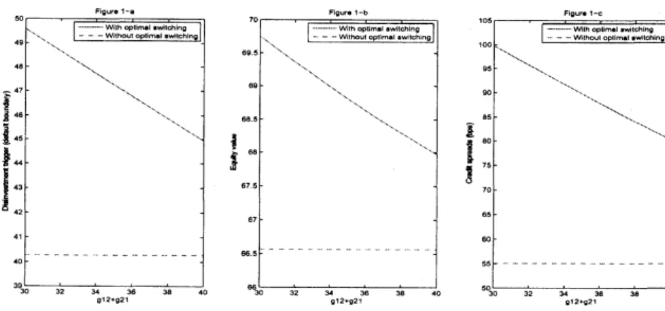
boundary, equity value, and credit spreads ofthe firm in regime 2.

$\ulcorner|9^{U\mathfrak{k}}\cdot t-\cdot$ so $\tilde{s}^{46}\overline{B}\ovalbox{\tt\small REJECT}_{45}^{47}$ $\xi_{u}$

1::

39 30 32 $u$ X38 $0$ 912.92$t$

Figure 1: The Impact ofconflicts of interestsondisinvestment trigger,equityvalue, and credit spreads.

7Depending on the bond covenants,the disposition ofassets might be restricted, especially before declaring

bankruptcy,asnoted bySmith andWarner (1979). Ifthis is thecaseand $x_{2}<d_{1}$, the optimal policy of equity

holderswillbesamewith thecaseof irreversibleinvestment,even thoughthe switchingcost$g_{21}$ is negative.Since

securing debt is not the mainissueofthispaper, weassumethat there isnorestriction regarding theinvestment

(12)

We

can see

in Figurel-athat$x_{2}(<d_{1})$decreases

as

investment reversibilityworsens, because

thefirm in regime 2 haslessincentiveto switch to regime 1

as

investment reversibility

worsens.

In Figure l-b,

we can see

that the equity valueofthe firm in regime 2 decreases

as

investment

reversibility worsens, which is

a

straightforward result, but is still higher than that without

optimal switching since the switching is implemented to maximize equity holders’ interest. We

canclearly seein Figure l-cthat the credit spreads of the firm withoptimal switching is higher

than those without optimal switching, and they decrease as investment reversibility worsens

because of the decrease inthe default boundary.

3.3 Overinvestment,

Underinvestment

Jensen and Meckling (1976) pointed out the overinvestment problem by showing that a firm

might be willing to accept projects with negative net present values if the expected payoff of

shareholders increases at the expense of creditors. Meanwhile, Myers (1977) demonstrated the

problem of underinvestment by showing that a firm financed with risky debt would pass up

valuable investment opportunities that could make a positive net contribution to the market

value of the firm. In this subsection, we capture both overinvestment and underinvestment

problems by comparing theinvestment trigger ofan unlevered firm andthat of

a

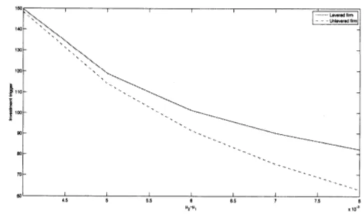
levered firm.

It is well known that equity holders are more likely to exploit projects at the expense of

creditors when the

new

projects

are

risky. To examine this problem,

we use

the benchmark

parameters except for$\sigma_{21}$ that

we

change from

0.2

to 0.25,

We

can

clearly

see

in Figure2 that the investment trigger of alevered firm is much lower than

that of an unlevered firm, which implies that the investment timing ofa levered firm is earlier

than that of an unlevered firm, and the problem exacerbates as the investment reversibility

lowers. Furthermore, the gap between two triggers widens

as

the difference of volatility in the

two regimes

increases.

This result reveals that equity holders

are

more

likely to invest in risky

projects when the firm is

a

levered one, shifting their risks to debt holders, and the problem

becomes

severe as

thegap ofvolatility increases.

$u$ tu ト

沖

$n$ $t\infty$

$|\cdot t$ $0t\infty$ $0,/$ $05$ 012 $,arrow 0,a$ $0ta$

$0\iota u$ $ot.$ $0\uparrow u$ 0/5

(13)

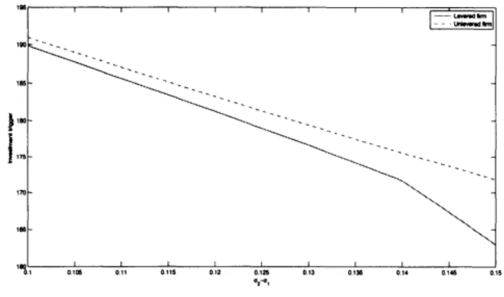
It is also known that equity holders may forgo profitable investment opportunities when

projects

are

not risky enough. To verify thisproblem,

we

suppose that $\mu_{1}=0.03,$$\sigma_{1}=\sigma_{2}=0.1,$

$g_{12}=10,$ $g_{21}=-9$, and let $\mu_{2}$ vary from 0.034 to 0.038. This assumption implies that it is

possibleto raise theexpected growth rate without raising volatility, which is ideal for creditors,

while it might not be for equity holdersthat bear the investment costs.

We can see in Figure 3 that the investment trigger of a levered firm is higher than that of

an unlevered firm, which implies that the firm defers timing of investment when debt is issued.

Moreover, the gap between two triggers widens as the differences in expected growth rates in

tworegimes increases. This result arises from the fact that only equityholdersbear the costs of

investment while profits from the investment areshared with debt holders.

Figure 3: Investmenttriggers representingunderinvestment problem.

4 Empirical Implications

In spite of the virtue of the theoretical backgrounds, structural models have been criticized for

thelack ofempiricalvalidity. This is because they usually do not providesufficient spreads, and

reduced-form models can be considered to avert this problem

as

they postulate credit events

exogenously so_{that the default time becomes totally inaccessible stopping time. In addition, the}

problem

can

be resolved in the framework of structural models by adopting jump diffusion

or

introducing imperfect information. Other research attempted to illustrate the spreads by

non-defaultcomponents,such

as

liquidity, taxes, call and conversion features,or

even

macroeconomic

conditions and the business cycle. In this section, we address how credit risk modeling with

optimal switchingcanenhance theempiricalvalidityof structuralmodels,especially interms of

the relationship between yieldspreads and credit grade of the bonds, based

on

various features

of the model that we have examined inthe previous section.

Jones et al. (1984) argue that the Merton (1974) model fits better for junk bonds since it has greater incremental explanatory power for riskier bonds. Huang and Huang (2002), who

empirically testedvariousstructural models, concluded that credit risks account for only asmall

(14)

fraction ofthe observed spreads forspeculative grade bonds. Eom et al. (2004) also empirically

analyzed various structuralmodels, andverifiedthat the spreads predicted by Leland andToft’s

(1996) model

are

often either ludicrously small

or

incredibly large. It is natural to deducethat

the ludicrously small and incredibly large spreads

are

generated from the bonds of speculative

grade and investment grade, respectively. They conclude that the crucial problem of structural

models that has to be

overcome

is to raise the average predicted spread relative to the model

ofMerton (1974), whichcannot generate sufficiently high spreads, without overstating the risks

associated with volatility, leverage,

or

coupon.

Asexplained before, default

occurs

only inregime 1 in

our

model. Hence,

we

can

regard the

bonds in regime 1 and regime

2 as

speculative grade and investment grade bonds, respectively.

To clarify the impactofoptimal switching

on

yield spreadsofspeculative bonds,let

us

compare

yield spreadsof the firmin regime1with optimal switching and those without optimal switching.

We

use

the benchmarkparametersexceptfor$g_{21}=-10$toreflect the lowinvestmentreversibility

in the real world.

We can see in Figure 4 that the yields of the firm in regime 1, i.e. those of speculative

grade bonds, with optimal switching

are

lower than the yields without optimal switching. This

is because the default boundary ofa firm with an option to invest is lower than that without

the option. Note that thedefault boundary decreases

as

regime 2 becomes more profitablefor

equity holders, as weexamined in the comparative statics.

Figure 4: Creditspreadsofspeculative grade bonds.

Next,

we

investigate yield spreadsof investment grade bonds,i.e. those ofthefirm inregime

2. We use the same parameters

as

in the former case.

Figure5 shows that theyieldspreads of the firm in regime 2 withoptimal switchingishigher

than the yield spreadswithout optimal switching. This result arises from the agencyproblemof

debt combined with the firm’s option todisinvest, that is,defaultof the firm right after switching

to regime 1. Note that thisproblemis

more

likely to

occur

when investment reversibility islow.

Considering that almost

none

of the investment projects

are

perfectly reversible in the real

world, it is reasonable to consider the agency problem of debt

as one

of the factors that raises

(15)

debt to explain the observed yields that are much higher than yields generated from Leland

(1994), but the effects were insignificant. In contrast, the impact of agency problems on

our

modelis considerable.

Figure 5: Creditspreadsof investment grade bonds.

Combining these results, we can resolve the problem of structural models pointed out by

Jones et al. (1984), Huang and Huang (2002), and Eom et al. (2004), i.e. wide variations in

yield spreads dependingon the credit gradeof bonds. Yield spreadsofspeculative grade bonds

decrease from the firm’s option to invest, while those ofinvestment grade bonds increase from

agencyproblems combined with the firm’s option to disinvest.

5 Conclusion

In this paper,we proposedthe credit riskmodelwithoptimal switching between twodifferent

dif-fusion regimes. By allowing negative switchingcost, we canintegrate awide rangeof investment

reversibility inthe framework. The default boundary andswitching thresholds

are

endogenously

determined, and wepresented comparative statics regarding diffusion regimes, switching costs,

and investment reversibility. Conflicts of interests between shareholders and creditors appear,

andboth overinvestment and underinvestment problems

are

examined bycomparing investment

triggers ofan unlevered firm andalevered firm. Basedon these features,

our

modelresolves the

problem of structural models pointed out by Jones et al. (1984), Huang and Huang (2002), and

Eom et al. (2004), namely, the wide variations in yield spreads depending on the credit grade

of the bonds. The yield spreads of speculative grade bonds decrease since the default boundary

lowers because of an option to invest, and those of investment grade bonds increase because of

agencyproblems combined with

an

optionto disinvest.

References

[1] Abel, A.B., Eberly, J.C.,

1996.

Optimal Investment with Costly Reversibility. Review of

(16)

[2] Bayraktar, E., Egami, M., 2010. Onthe One-dimensional OptimalSwitching Problem. Math-ematics of Operations Research 35, 140-159.

[3] Black, F., Scholes, M., 1973. The Pricing

_of

Options and Corporate Liabilities. Journal of

Political Economy 81, 637-654.

[4] Brekke, K.A., $\emptyset$ksendal, B., 1994. Optimal Switching in an Economic Activity under

Uncer-tainty. SIAM Journal

on

Control and optimization 32,

1021-1036.

[5] Brennan, M.J., Schwartz, E.S.,

1985.

Evaluating Natural Resource Investments. Journal of

Business 58, 135-157.

[6] Childs, P.D., Mauer, D.C., 2008. Managerial Discretion, Agency Costs, and Capital

Struc-ture. Working paper.

[7] Dixit, A.K.,

1989.

Entry and ExitDecisions under Uncertainty. Journal of Political Economy

97,

620-638.

[8] Djehiche, B., Hamad\’ene, S., Popier, A., 2009. A Finite Horiizon Optimal Multiple Switching

Problem. SIAM Journal on Control and optimization 48,

2751-2770.

[9] Duckworth, K., Zervos, M.,

2001.

A Model

_for

Investment Decisions with Switching

Costs.

The Annals ofApplied Probability 2001,

239-260.

[10] Duffie, D., Lando, D., 2001. Term Structures

_of

Credit Spreads with Incomplete Accounting

Information.

Econometrica69, 633-664.

[11] Eom, Y.H., Helwege, J., Huang, J.,2004. Structural Models

_of

Corporate BondPricing:$An$

Empirical Analysis. The Review of Financial Studies 17,

499-544.

[12] Ericsson, J.,2000. Asset Substitution, Debt Pricing, Optimal Leverage and Maturity.

Work-ing paper.

[13] Guo, X., Miao, J., Morellec, E.,

2005.

Irreversible Investment with Regime

_Shifts.

Journal

of

Economic

Theory 122,

37-59.

[14] Hackbarth, D., Miao, J., Morellec, E.,

2006.

Capital Structure, CreditRisk, and

Macroeco-nomic Conditions. Journal of Financial Economics 82, 519-550.

[15] He, Z.,2011.A Model

_of

DynamicCompensation andCapitalStructure. Journal of Financial

Economics 100,

351-366.

[16] Huang, J., Huang, M., 2002. How Much

_of

the Corporate $\mathcal{I}$Veasury YieldSpread Is Due to

Credit Risk$(?$

Working paper.

[17] Jeon, H., Nishihara, M., 2013. Credit Risk Model with Optimal Switching. Working paper.

[18] Jensen, M.C., Meckling, W.H.,

1976.

Theory

_of

The Firm: Managerial Behavior, Agency

(17)

[19] Jones, E.P., Mason, S.P., Rosenfeld, E.,1984. Contingent Claims Analysis

_of

Corporate

Capital Structures: An EmpiricalInvestigation. The Journal of Finance 39, 611-625.

[20] Leland, H.E., 1994. Corporate Debt Value, Bond Covenants, and Optimal CapitalStructure.

The Journal of

Finance

49,

1213-1251.

[21] Leland, H.E., 1998. Agency Costs, Risk Management, and Capital Structure. The Journal

of Finance 53, 1213-1243.

[22] Leland, H.E., Toft, K.B., 1996. Optimal Capital Structure, Endogenous Bankruptcy, and

the Term

Structure

_of

CreditSpreads. The Journal of Finance 51, 987-1019.

[23] Merton, R.C., 1974. On The Pricing

_of

Corporate Debt: The Risk Structure

_of

Interest

Rates. The Journal of Finance 29, 449-470.

[24] Myers, S.C., 1977. Determinants

_of

Corporate Borrowing. Journal of Financial Economics

5, 147-175.

[25] Pham, H., 2009.

Continuous-time

Stochastic Control and optimization with Financial

Ap-plications. Springer.

[26] Pham, H., Vath, V.L., Zhou, X.Y., 2009. Optimal Switching overMultiple Regimes. SIAM

Journal

on

Control and optimization 48,

2217-2253.

[27] Smith, C.W., Warner J.B.,

1979.

On Financial Contracting: An Analysis

_of

Bond

Covenants. Journal of Financial Economnics 7, 117-161.

[28] Vath, V.L., Pham, H., _2007. Explicit Solution to an Optimal Switching Problem in the

Two-regime Case. SIAM Journal on Control and optimization 46, 395-426.

[29] Zervos, M.,

2003.

A Problem

_of

Sequential Entry and Exit Decisions Combined with