A numerical level set method for the Stefan problem with a crystalline Gibbs-Thomson law (The State of the Art in Numerical Analysis : Theory, Methods, and Applications)
9
0
0
全文
(2) 138 to change the phase per unit volume is given by the specific latent heat of phase transition L , and this energy is delivered by the heat flux -k\nabla u . This problem appears in models. of dendritic growth and solidification. For a more detailed discussion, see [ C_{-}\backslash IOS , BGN] and the survey article [Ga] and the references therein.. 2. Crystalline mean curvature. Following [AG, T ], the crystalline mean curvature can be introduced as the first variation of the anisotropic surface energy functional defined for any sufficiently smooth set U\subset \mathbb{R}^{n} as. \mathcal{F}(U):=\int_{\partial U}\sigma(\nu)dS, where. \sigma. : \mathcal{S}^{n-1}arrow(0, \infty) is a given anisotropy. For the detailed overview of this topic,. see the survey [B] or [Gu, GG, GP1, homogeneously to whole. \mathbb{R}^{n}. C_{\perp}\backslash IP ].. In what follows we extend. \sigma. positively one‐. as. \sigma(p)=\{ begin{ar ay}{l} |p\sigma(\frac{p}{|p}), p\neq0, 0, p=0. \end{ar ay} We will assume that the extended. The anisotropy. \sigma. \sigma. is convex.. determines the optimal crystal shape (Wulff shape), that is, the. shape that minimizes the anisotropic surface energy among shapes with the same volume as. \mathcal{W}:=\{x:x\cdot p\leq\sigma(p), p\in \mathbb{R}^{n}\} ,. (2.1). see [T]. If \sigma is smooth on \mathbb{R}^{n}\backslash \{0\} and \{p:\sigma(p)\leq 1\} is a strictly convex bet, and \partial U is smooth, the first variation of \mathcal{F} with respect to a change of volume is div_{\partial U}(\nabla\sigma(\nu)) , where div_{\partial U}. is the surface divergence, see [I3]. We define. \kappa_{\sigma}:=-div_{\partial U}(\nabla\sigma(y)) .. (2.2). We are, however, specifically interested in anisotropies that are not smooth, in particu‐ lar whose level set \{\sigma\leq 1\} is a convex polytope and \mathcal{W} above is the dual convex polytope. [R]. In other words, when. \sigma. \mathbb{R}^{\eta}arrow[0, \infty ) is a convex, piece‐wise linear function. We. call such anisotropies crystalline. In this case, the definition of \kappa_{\sigma} becomes much more involved since \nabla\sigma(\nu) is no longer defined pointwise and might be discontinuous even on. a smooth surface. A natural generalization of (2.2), consistent with the general abstract theory of monotone operators due to Kōmura and Brézis [K, B_{1}] , is to replace the first variation of \mathcal{F} with a subdifferential on an appropriate Hilbert space. This leads to the. definition [I3, ChIP, GP1] \kappa_{\sigma}:=-div_{\partial U}z_{\min}, where z_{\min} is the element of the set. \{z\in L^{\infty}(\partial U) : z\in\partial\sigma(\nu), divz\in L^{2}(\partial U)\}. (2.3).
(3) 139 that minimizes. \Vert divz\Vert_{L^{2}(\partial U)} ,. if the set is nonempty. Here \partial\sigma is the subdifferential of. \sigma,. \partial\sigma(p):=\{\xi\in \mathbb{R}^{n}:\sigma(p+h)-\sigma(p)\geq\xi\cdot h, h\in \mathbb{R}^{n}\}. While. might not be unique, divz_{\min} is. Unfortunately, even for smooth. z_{\min}. set (23) might be empty, in which case. \kappa_{\sigma}. \partial U. the above. is not defined.. We call such \kappa_{\sigma} the crystalline mean curvature of \partial U . This quantity enjoys a number of interesting properties, including the comparison principle. Furthermore, it is a singular, nonlocal quantity on the surface \partial U . In particular, if \partial U has a flat part, called a facet, with normal \nu such that \sigma is not differentiable at \nu, \kappa_{\sigma} then depends on the shape of the facet. For example, in dimension n=2 , facets of U are line segments, and on each of them \kappa_{\sigma} is a constant that is inversely proportional to their length.. The well‐posedness of (1.1) with a crystalline \sigma seems to be open. A general theory of solutions for the crystalline mean curvature flow (3. ı) has been available only recently [CMP, CAINP, GP1, GI^{\supset}2 ].. 3. Numerical algorithm. There have been many very successful algorithms developed to solve (1.1) with a smooth \sigma numerically and listing them all is beyond the scope of this note. One of the difficulties is the unstable nature of the dendritic growth and an extra care must be taken to avoid the discretization and the choice of a mesh to produce unwanted artifacts. See [C_{-}^{1}\backslash 1OS,. BGN, Ga] and the references therein. In this work to treat the crystalline mean curvature directly without any regularization, we instead use the algorithm proposed by [O()TT] that relies on the split Bregman iteration scheme introduced in [G()] to efficiently find minimizers of anisotropic total variation functionals. This approach builds on the level set. formulation due to Chambolle [C] of the minimizing movements time semidiscretization of the anisotropic mean curvature flow. V=\beta(\nu)(\kappa_{\sigma}+f). on. (3.1). \partial E. by Almgren, Taylor and Wang [ATW]. In this algorithm, we fix a computational domain \Omega\subset \mathbb{R}^{n.} sufficiently large so that E_{t}\subset\Omega for all t\in[0, T] for some fixed T>0 , and choose a time step h>0 . Then we approxilnate E_{t_{\gamma\eta} , t_{m}=mh, m=1,2, , by a sequence of sets E_{m}\subset\Omega , where E_{m} :=\{x : v_{m}(x)<0\} , and v_{m}\in L^{2}(\Omega)\cap BV(\Omega) is the minimizer of thc functional \cdots. J_{m}(v) := \frac{1}{2h}\Vert v-w_{m}1\Vert_{L^{2} ^{2}+\int_{\Omega} \sigma(\nabla v)dx-\{v, f_{m}\rangle_{L^{2} . Here \beta,. w_{m-1}. is the signed distance function to the set E_{m-1} with respect to the anisotropy. w_{m-1}(x)=signdist_{\beta}E_{m-1}(x):=\dot{ \imath} nf\beta^{\circ}(x-y)-\dot{ {\imath} n_{c}f\beta^{\circ}(y-x)y\in E_{n1-1}y\in E_{m-1} where \beta^{\circ} is the polar of \beta[R],. \beta^{\circ}(x):=\sup\{\frac{x\cdot\nu}{\beta(\nu)}:\nu\in S^{n-1}\}.. ’.
(4) 140 The minimizer of J_{m} can be found efficiently by the split Bregman minimization. method of [GO] as observed in [OOTT]. We proceed by introducing a new variable \mathbb{R}^{n}arrow \mathbb{R}^{n}. d=\nabla v. d. :. that is then relaxed by a L^{2} ‐penalization term.. and add a constraint In other words, we choose \lambda>0 and in place of J_{m} we minimize. \tilde{J}_{m}(v, d) :=\frac{1}{2h}\Vert v-w_{m-1}\Vert_{L^{2} ^{2}+ \int_{\Omega}\sigma(\nabla v)dx-\{v, f_{m}\}_{L^{2} +\frac{\lambda}{2}\Vert d- \nabla v\Vert_{L^{2} ^{2} Since alı the terms are convex, we can attempt to find the minimizer by alternatively minimizing with respect to v and d . This produces a sequence converging to the unique minimizer of \tilde{J}. . However, this minimiLer does not generally satisfy d=\nabla v and therefore is not a minimizer of J_{m}.. This is addressed by introducing a third variable b : \mathbb{R}^{r\iota}arrow \mathbb{R}^{n} that accumulates the ‘error \nabla v-d during the iteration. The full algorithm can be stated as follows: Set b_{m,0}=d_{m,0}=0 and for k=0,1 , . . . iterate \cdot,. v_{m,k+1} arrow\arg\min_{v}\frac{1}{2h}\Vert v-w_{m-1}\Vert^{2}-\{v, f_{m}\}+ \frac{\lambda}{2}\Vert d_{m,L}-\nabla v-b_{m,k}\Vert^{2} d_{m,k+1}arrow\arg_{d}nlin \int_{\Omega}\sigma(d)dx+\frac{\lambda}{2}\Vert d-\nabla v_{m_{\dot{r} k}- b_{m,k}\Vert^{2} b_{m,k+1}arrow b_{m,k}+\nabla v_{m,k+1}-d_{m,k+1} ,. (3.2a) (3.2b) (3.2c). until convergence is achieved, for instance, until \Vert v_{m.k+1}-v_{m,k}\Vert is sufficiently small. This algorithm converges to a stationary point, see [G()] . When that happens, we deduce from the third step (3.2c\cdot) that the limit (v_{m}, d_{m}, b_{m}) satisfies \nabla v_{m}=d_{m} and therefore v_{m} is the unique minimizer of J_{m} . In particular, it does not depend on the choice of \lambda . However, \lambda influences the difficulty to solve the minimization problem (3.2_{c}) and the overall speed of convergence.. Note that solving (3.2a) is equivalent to solving a linear elliptic partial differential equation for v , while solving (3.2b) after discretization yields a completely decoupled minimization problem at each node, which only requires evaluating the projection on the. optimal shape \mathcal{W} in (2.1). See [GO, OOTT] for more details. To couple this scheme with the heat equation in (1.1), we interpret the second equation in (] 1) as an energy source concentrated on the surface \partial E and add it to the heat equation:. u_{t}=div(k\nabla u)+LV\mathcal{H}^{n-1}\lfloor\partial E_{f}. After tiıne discretization, for each m=1,2 ,. we. 1. solve for E_{m} using the above algorithm with f_{m}=-\alpha^{-1}u_{7n-1} (in the TV minimiza‐ tion, we take \overline{\beta}=aE with \beta from (1.1)), and then 2. solve for the solution u_{7\eta} of. u_{m}-hdiv(k\nabla u_{m})=u_{m-1}+hLV_{m}\mathcal{H}^{n-1}\lfloor\partial E_{m} ,. (3.3). where the nonnal velocity V_{m} is estimated using the value of the signed distance function signdist E_{m-1} with respect to the usual Euclidean metric on the set \partial E_{m} as. hV_{m}= signdist E_{m-1}..
(5) 141 141 We discretize both (3.2) and (33) by the standard piece‐wise linear finite elements on a regular triangular grid in two dimensions or a regular tetrahedral grid in three. dimensions [P]. The discrete signed distance function is computed using the fast sweeping algorithm [Z] with the initialization scheme proposed in [P] Recomputing the signed distance function necessarily moves the level set and intro‐ duces an error. However, we observe that v_{m} is still very close to a distance function of E_{m} near its boundary and therefore we usually set w_{m}=v_{m} . We recompute the actual signed distance function using the fast sweeping algorithm only after a prescribed number of steps. It would be more appropriate to set the value of f_{m} using the extension of the value. of-2L_{m-1}|_{\partial E_{m-1}} via a transport equation as in [AS] to increase the accuracy and reduce. the need to reinitialize the distance function. This will be explored in the future. It is natural to consider an adaptive mesh or perform the computation only near the boundary of the evolving domain. This is a subject of ongoing work.. 4. Numerical results. In this section we present results of a few simple numerical experiments using the above algorithm, see Figures 1‐4.. (- \frac{1}{2}, \frac{1}{2})^{2} for the total variation domain \Omega_{heat}=\{x\in \mathbb{R}^{2} |x|<\frac{1}{2}\}. We fix the domain \Omega=. minimization and the fast. sweeping method, and the for the heat equation. The boundary data for the hcat equation is set to -10^{-3} . For the mobility, we always use \beta(p)=100|p|_{2} . The conductivity is taken to be 1 outside the crystal and 0 inside. We discretize the domain by subdividing it uniformly into 256^{2} squares and split each of those in half to produce the triangular mesh. The time step is fixed at \tau=2.5\cross 10^{-4}. Larger time steps lead to instability, most likely due to the explicit nature of the coupling of the heat equation with the anisotropic mean curvature flow. The optimal choice of the parameter \lambda is an interesting problem. In the original paper. [GO] for total variation denoising applications, the value. \lambda=\frac{2}{h} was used. However, in the. current computations the value \lambda=\frac{1}{10h} was found using numerical experiments to provide a significant speed‐up of the convergence. With this choice, only about 3‐5 iterations of. the aıgorithm (3.2) per time step are needed, and each of the presented results takes 15−30 minutes to compute on an Intel Core i7‐4770K processor. The simple nuınerical results show that the method can reproduce facet breaking due to the uneven cooling of the facets, and that neighboring crystals do not merge because the diffusion is limited inside the crystal. Due to the technical limitations of the current implementation, thc fixed boundary for the heat equation is relatively close to the growing crystaı, and this leads to a strong forcing at thc exposed vertices. The facets there are therefore short and the crystal surface is not fully faceted. On the other hand, this illustrates that the method is capable of handling not fully faceted crystals, which is observed in practice in such strongly forced situations. In summary, the initial implementation produces promising results, but more work is needed to make it competitive with other available algorithms. Adaptive meshes, a more accurate treatment of the boundary forcing term in the level set method and various other improvenlents are being consideied. In particular, a tılree dimensional simulation is in preparation..
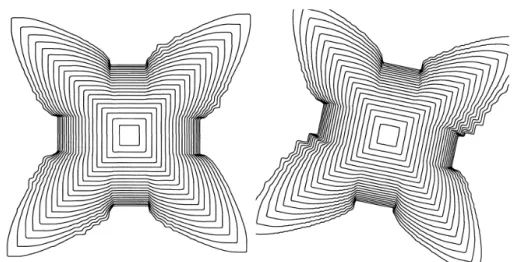
(6) 142. Figure 1: The evolution of a single square crystal of initial side length 0.05 growing with \alpha=5\cross 10^{-7} , plotted at 2 second intervals aligned with the mesh (left) and rotated by. 0.2 radians (right).. Figure 2: The evolution of a single square ciystal of initial side length 0.05 growing with \alpha=10^{-8} , plotted at 2 second intcrvals aligned with the mesh (left) and rotated by 0.2 radians (right). Since the curvature effect is significantly weaker than in Figure 1, only. short facets appear in regions with a relatively weak forcing. The effect of the mesh is more pronounced: the dendrites splitting in half along the diagonal directions are almost certainly mesh artifacts..
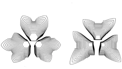
(7) 143. Figure 3: The evolution of a single hexagonal crystal of initial side length 0.05 growing with \alpha=2.5\cross 10^{-7} (left) and \alpha=10^{-8} (right), plotted at 2 second intervals. The horizontal dendrites grow faster, indicating an anisotropy caused by the mesh.. Figure 4: The evolution of three initially hexagonal or square crystals growing with a 5\cross 10^{-7} , plotted at 2 second intervals. Note that the crystals do not merge.. =.
(8) 144 Acknowledgments The work of the author is partially supported by JSPS KAKENHI Grant No. 26800068. (Wakate B).. References [AS] D. Adalsteinsson and J. A. Sethian, ’l’he fast construction of extension velocities in level set methods, J. Colnput. Phys. 148 (1999), no. 1, 2‐22, DOI 10. 1006/ jcph.199S.6090.. [A'\perp'11^{\gamma}] F. Alın glen, J. E. Taylor. and L. Wang, Curvature‐driven flows: a variational approach, SIAM J. Control Optiın . 31 (1993), no. 2, 387 43S , DOI 10.1137/0331020. [AG] S. Angenent and M. E. Gurtin, Multiphase thermomechanics with interfacial structure. II. Evo‐ lution of an isothermal interface, Arch. Rational Mech. Anal 108 (1989)_{\backslash }, no. 4, 323‐391, DOI 10.1007/BF0l04ı068. [BGN] J. W. Barrett. H. Garcke, and R. Nürnberg, Finite‐element approximation of one‐sided Ste‐ fan problems with anisotropic, approximately crystalline, Gibbs‐i homson law, Adv. Differentia] Equations 18 (2013)_{\dot{i}} no. 3 ‐ 4_{\dot{}}383-432.. [B] G. Bellettini, Art introduction to anisotropic and crystalline mean curvature flow_{\mathfrak{i} Hokkaido Univ. Tech. Pep. Ser. in Math. 145 (2010), 102 162. [Br] H. Brézis, Monotonicity methods in Hilbert spaces and some applications to nonlinear partial d_{iffe7} ential equations, Contributions to nonlinear functionaı anaıysis (Proc. Sympos. hIath. Res. Center, Univ. Wisconsin, Madison, Wis., 1971), Acadelnic Press, New York, 1971, pp. 10ı‐l56.. [C] A. Chalnbolle, An algorithm for mean curvature motion, Interfaces Free Bound. 6 (2004), no. 2, 195‐218, DOI 10. 4171/IFB/97. [CMNP] A. Chanlboıle, M. Morini, M. Novaga, and M. Ponsigıione, Existence and uniqueness for anisotropic and crystalline mean curvature flows, preprint, avaiıable at 4^{\sim}.1_{\xi^{\overline{y}_{\sim^{\backslash :\prime}}^{\backslash } }/cZx^{ -}c\ddot{c}^{v} abs_{/}^{/}1702 03094. .. [CMP] A. Chambolle, M. Morini, and M. Ponsiglione, ETistence and Uniqueness for a Crystalline Mean Curvature Flow, Comın. Pure Appl. NIath. 70 (2017), no. 6, DO110. 1002/cpa.21668. [CMOS] S. Chen, B. IsIerriınan, S. Osher, and P. Slnereka, A simple level set method for solving Stefan problems, J. Conlput. Phyb. 135 (1997), no. 1_{\backslah,\prime} S‐29, DOI 10.1006/jcph.ı997.ó72l I\backslash IR1461705 [Ga] H. Garcke, Curvature driven interface evolution, Jalnesbel. Dtsch. Math.‐Vel. 115 (2013), no. 2, 63‐100, DOI 10.1365/sl329l‐0l3‐0066‐2.. [GG]. I\backslash I .‐H. Giga and Y. Giga, Evolving graphs by singular weighted curvature, Arch. Rational Mech Anal. 14ı (1998) no. 2, 117‐198.. [GP1] Y. Giga and N. Požáı, A level set crystalline mean curvature flow of surfaces, Adv. Differential Equations 21 (2016), no. 7‐8, 631‐698. [GP2] —, Approximation of general facets by admissible facets for anisotropic total variation energies and its application to the crystalline mean curvature flow, Connn. Pure Appl. Math.. (to appear). [GO] T. Goldstein and S. Osher, 7 he split Breqman method for Ll‐regularized problems_{i} SIAM J. Iınaging Sci. 2 (2009) , no. 2_{i}323-343_{:} DOI 10.1137/080725891 [Gu]. L I.. E. Guitin. Thermomechanics of evolving phase boundaries in the plane, Oxford Mathelnatical. hI_{oll}ograp1_{1}s , The Clarendon Press, Oxfoid Univeısity Press, New York, 1993.. [K] Y.. K_{\overline{O}1} nura,. Nonlinear semi‐groups in Hilbert space, J. Math. Soc. Japan ı9 (1967), 493‐507.. [P] N. Požár, On the self‐similar solutions of the crystalline mean curvature flow in three dimensions (in preparation)..
(9) 145 [OO 1^{\urcorner\ulcorner}1^{\urcorner}] A. Obernlan, S. Osher, R. Takei, and R. Tsai: Numerical methods for anisotropic mean curvature flow based on a discrete time variational formulation, Connnun. Math. Sci. 9 (2011), no. 3, 637 662, DOI 10 4310/CMS 2011. v9.\Pi 3 . al.. [Ft] R. T. Rockafellar, Convex analysis, Princeton Mathelnatical Series, No. 28, Princeton University Press, Princeton,. N. J., 1970. MR0274683 (43\# 445). [T] J. E. Taylor, Constructions and conjectures in crystalline nondifferential geometry. Differential geonnetry, Proceedings of the Conference on Differential Geolnetry, Rio de Janeiro (B. Lawson alld K. Tanenblat, eds.), Pitman Monogr. Surveys Pure Appl. \beta_{\backslash }Iath_{:} vol. 52, Longnlan Sci. Tech., Harlow, 1991, pp. 321‐336, DOI 10.1111/j.l439‐0388.l99l tb00191 x.. [Z] H. Zhao, A fast sweeping method for eikonal equations, Math. Coınp. 74 (2005), no. 250, 603‐ 627, DOI 10.1090/S0025‐57l8‐04‐0l678‐3.. Faculty of Mathematics and Physics Institute of Science and Engineering Kanazawa University Kakuma town, Kanazawa Ishikawa 920‐1192 JAPAN. E‐mail address: [email protected]‐u.ac.jp.
(10)
図
関連したドキュメント
She reviews the status of a number of interrelated problems on diameters of graphs, including: (i) degree/diameter problem, (ii) order/degree problem, (iii) given n, D, D 0 ,
В данной работе приводится алгоритм решения обратной динамической задачи сейсмики в частотной области для горизонтально-слоистой среды
Keywords: continuous time random walk, Brownian motion, collision time, skew Young tableaux, tandem queue.. AMS 2000 Subject Classification: Primary:
VARIATIONAL AND NUMERICAL ANALYSIS OF THE SIGNORINI’S CONTACT PROBLEM IN VISCOPLASTICITY WITH DAMAGE
Sofonea, Variational and numerical analysis of a quasistatic viscoelastic problem with normal compliance, friction and damage,
We present sufficient conditions for the existence of solutions to Neu- mann and periodic boundary-value problems for some class of quasilinear ordinary differential equations.. We
Transirico, “Second order elliptic equations in weighted Sobolev spaces on unbounded domains,” Rendiconti della Accademia Nazionale delle Scienze detta dei XL.. Memorie di
We provide an efficient formula for the colored Jones function of the simplest hyperbolic non-2-bridge knot, and using this formula, we provide numerical evidence for the
We have introduced this section in order to suggest how the rather sophis- ticated stability conditions from the linear cases with delay could be used in interaction with
