A Note on Idempotent Monomial Clones : Two is Strong; One is Weak (Developments of Language, Logic, Algebraic system and Computer Science)

全文

(1)64. 数理解析研究所講究録第2051巻 2017年 64-69. A Note. on. Two is. —. Monomial Clones. Idempotent. Hajime Machida. Strong; One. is Weak. Jovanka Pantovič $\dag er$. *. Tokyo, Japan. Novi. —. Csaba Szabó 8. Sad, Serbia. Budapest, Hungary. Abstract. polynomials are considered over Galois field \mathrm{G}\mathrm{F}(k) In particular, the generated by 2‐variable idempotent polynomials is the target of our study. Our results include that the clone generated by x^{2}y^{k-2} is the largest among all such clones and the clone generated by xy^{k-1} is the smallest among all such clones. Hence, observing the exponent of one variable, two is strong and one is weak. Clones of. .. class of clones. Keywords: clone; monomial clone; lattice of. clones. $\dag er$ $\d ag er$. Preliminaries. 1. Let k> 1 be fixed and. E_{k}=\{0, 1, . . . , k-1\}. functions defined. E_{k} that is, the. over. ,. set of functions defined set. \mathcal{J}_{k} of projections. always. over. E_{k} i.e., ,. A clone. by. set of maps from. \displaystyle \ovalbox{\t \smal REJECT} k=\bigcup_{n=1}^{\infty}\mathcal{O}_{k}^{(n)}. \mathcal{J}_{k}. by \mathcal{L}_{k}. A. .. for n\geq 1 the set of. into. E_{k}. .. Also, O_{k}. n‐variable. denotes the. special class of functions. is the. \mathcal{O}_{k}^{(n)}. which. is the function in. e_{i}^{n}. .. arbitrary. sum. for. some. As. a. over. E_{k} forms. a. It is well‐known that the lattice. field K and. of terms, that. of. one. e_{1} ,. special. .. .. .. ,. a. an. \mathcal{L}_{k} for k. positive integer. ( ‐variable). monomial. a. .. cardinality. of the. n,. an. ( n‐variable) polynomial. over. K is. a. is,. n. a\in K and i_{1} ,. has the. > 2. over. n. .. .. .. x_{n}^{i_{n}. ‐tuple (il,. K is. i_{n} ). in the \mathrm{s}\mathrm{p}\mathrm{e}(_{J} ified range.. an n ‐variable. polynomial consisting. .. .. .. term, i.e.,. some. and. lattice with respect to inclusion and is. extremely complex.. e_{n}\in \mathrm{N} and a_{i_{1_{j}}\ldots,i_{n}} \in K for each. case,. (functional) composition. subset C of 0_{k} which is closed under. a. The set of clones. .. \displaystyle \sum_{0\leq i_{1}\leq e_{1},\ldots,0\leq i_{n}\leq e_{n} a_{i_{1},\ldots,i_{n} x_{1}^{i_{1}. *. E_{k}^{n}. ,. continuum and its structure is. for. \mathcal{O}_{k}^{(n)}. for any n>0 and 1\leq i\leq n where. e_{i}^{n}. E_{k} is. over. denoted. For. Denote. takes the value of the i‐th variable.. includes. finite. .. .. .. ,. machida.zauber@gmail.com. x_{1}^{i_{1} \cdots x_{n}^{i_{n}. i_{n}\in \mathrm{N}. $\dag er$. pantovic@uns.ac.rs. $\d ag er$ csaba@cs.elte.hu. ,.

(2) 65. For. the structure of. Property Hence,. For. a. denoted. defined. An. 2:. n ‐variable. a\in \mathrm{G} $\Gamma$(k). some. x\in \mathrm{G}\mathrm{F}(k). For every. 1:. and. subset S of. by (S}.. study of monomial as. r_{1}. \{f\}. =. .. ,. .. generated by. any. over. polynomial. a. ,. E_{k}. ,. ,. for n>0 , is. r_{n} with 0<r_{1}. is. a. \{S\}. .. ,. .. .. ,. function. n ‐variable. is the smallest clone. by \langle f\rangle. if C. is. motivated. partly. a. in. E_{k}. Let. .. a. monomial clone. Throughout. the. by. consider. we. f. defined. E_{k}. over. be. the rest of the paper,. generated by. generated by. Monomials stated. above,. the variable. a. a. over. E_{k}. .. some. monomial. produced. The. proof is. from monomials. If C. is minimal in the set. is said to be. s. we. consider 2‐variable. Hereafter, by. them.. f(a\ldots., a)=a ovcr \mathrm{G}\mathrm{F}(k) i_{j}\equiv 1 (\mathrm{m}\mathrm{o}\mathrm{d} k-1) (We. idempotent if f. satisfies. monomial with coefficient 1. idempotent. idempotent. monomials. monomial clone. a. .. .. monomial. Let. us. we. shall. denote. over. E_{k}. mean a. by \mathcal{M}_{k}. the. E_{k}.. x^{s}y^{t} we. consider 2‐variable monomials .. symbols.) Clearly,. when the exponents. and t. (For. convenience. s+t=k is. satisfy. an. x^{S}y^{t}. we use x. equivalent. for. 0 < s, t < k with the. and y instead of x_{1} and x_{2} , for ,. condition for. x^{8}y^{t}. to be. idempotent. 0<s, t<k.. is. a. monomial which generates. must be. a. 2‐variable monomial. m. of monomial. limited class of monomials and monomial clones. an n ‐varíablc. 2‐variable. over. additional condition s+t=k. (1). x_{n}^{r_{n}. Monomial Clones. set of such monomial clones. If. .. containing S and. following property.. m is idempotent if and only if \displaystyle \sum_{j=1}^{n} idempotent for polynomials in an obvious way.). monomial clone. m. .. (in \mathcal{L}_{k} ).. m=x_{1}^{i_{1}}\cdots x_{n}^{i_{n}}. and monomial clones. Note:. .. A monomial clone is. .. generated by. monomial cannot be. Evidently (by Property 1),. was. axí1. as. them.. abuse the term. As. expressed. r_{n}<k.. is denoted. monomial clone. which is not. minimal clone. Idempotent. 2.1. ex‐. finite field.. a. x^{k}=x.. \mathrm{G}\mathrm{F}(k). m over. .. the clone. clones is. In the rest of the paper. a. It is. .. uniquely. is. of composition.. clones then C is. for all. basic property of. ,. Lemma 1.1 Let C be. An. \mathrm{G}\mathrm{F}(k). is. a. \mathrm{G}\mathrm{F}(k). the Galois field over. introduce. us. C=\langle m\rangle.. ,. means. 2. as. defined. \mathcal{O}_{k} the clone generated by S. When S. E_{k} i. e.,. immediate. by. E_{k}. x_{n}\rangle. following. it holds that. monomial. integers. Definition 1.1 A clone C. The. ,. let. e,. follows.. as. m over. \mathrm{G}\mathrm{F}(k). \ldots. positive integer. a. treat. we. f(x_{1},. The. .. p and. have:. we. Property for. over. ,. function. n‐variable. polynomial. as a. prime. a. E_{k} that is,. finite ỉield into. a. well‐known that any. pressed. i.e., k=p^{e} for. power k ,. prime. a. x^{s}y^{t}. a. non‐unary minimal clone. and. (2). (in \mathcal{L}_{k} ) then, clearly,. the condition s+t=k must be. satisfied,.

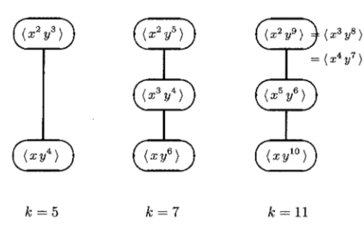
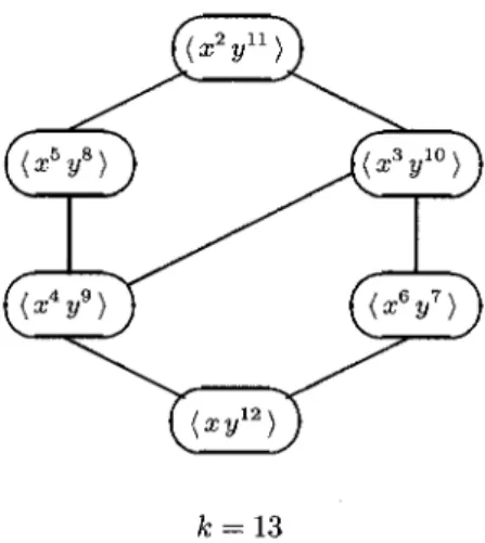
(3) 66. k=5. k=7. Figure since. \langle x^{s}y^{t}\rangle. 1: Monomial clones for k=5 ,. composition. The proof Lemma 2.1 For with. is. integers. u,. (i). v. satisfying. J_{k} ) by composition,. Lemma 2.2 Let k be. Proof. 11. a. s+t=k'. ). on. the exponents is. preserved by. straightforward.. Some easy consequences. (1). 7,. does not contain any non‐trivial unary functions.. The next lemma shows that the condition. (together. k=11. are. prime. i. e.,. 0 < u,. v. <. x^{u}y^{v}\in\{x^{S}y^{t}\rangle. ,. k,. if x^{u}y^{v}. then. we. is obtained. have. from x^{s}y^{t}. u+v=k.. presented. power. For clones. \{xy^{k-1}\}\underline{\subseteq} \{x^{2}y^{k-2}\}. on. GF(k). we. have the. following.. (2) \{x^{4}y^{k-4}\rangle\subseteq\langle x^{3}y^{k-3}). From. (k-2)^{2} = ((k-1)-1)^{2} \equiv 1 (\mathrm{m}\mathrm{o}\mathrm{d} k-1) it follows that. x^{2}(x^{2}y^{k-2})^{k-2}=x^{k-1}y.. (ii) Similarly,. (k-3)^{2} = ((k-1)-2)^{2} \equiv 4 (\mathrm{m}\mathrm{o}\mathrm{d} k-1) implies. 3 In. x^{3}(x^{3}y^{k-3})^{k-3}=x^{k-4}y^{4}.. Two is Figures. and 13.. \square. strong; One is weak. 1 and 2 the set. An observation. refer the exponents of. \mathcal{M}_{k} of. we. one. the monomial clones is shown for the. cases. get from these diagrams is the following (where. variable):. Two is strong and. one. is weak!. k=5 , 7, 11 two and. one.

(4) 67. Figure. Two is. 3.1. Proposition. 2: Monomial clones for k=13. strong. 3.1 For any. power k>1 and any 0<s<k , it holds that. prime. \langle x^{S}y^{k-s}\rangle \underline{\subseteq} \{x^{2}y^{k-2}\rangle. In other. words,. \{x^{2}y^{k-2}\}. Proof We shall prove Basis:. is the. largest. clone in. x^{S}y^{k-\mathrm{s}}\in\{x^{2}y^{k-2}\rangle for i.e., xy^{k-1}. The monomial with s=1 ,. ,. \mathcal{M}_{k}.. any. 0<s<k. by induction. is obtained from. x^{2}y^{k-2}. on s.. in the. following. way.. y^{2}(y^{2}x^{k-2})^{k-2} = x^{(k-2)^{2}}y^{2k-2} = xy^{k-1} Thus. we. have. Inductive and. x^{S}y^{k-s}\in\langle x^{2}y^{k-2} ). Step:. x^{2}y^{k-2}. as. for s=1 , 2.. \displayst le\mathrm{L}\frac{k}2\rflo r. $\Gamma$ \mathrm{o}\mathrm{r} any 1 < t <. ,. we. obtain. x^{2t-1}y^{k-2\mathrm{s}+1}. and. x^{2t}y^{k-2s}. from. x^{t}y^{k-t}. shown below.. \left\{ begin{ar ay}{l} (x^{t}y^{k-t})^{2}x^{k-2}=x^{2t+k-2}y^{2k-2t}&=x^{2t-1}y^{k-2t+1}\ (x^{t}y^{k-t})^{2}y^{k-2}=x^{2t}y^{3k-2t-2}&=x^{2t}y^{k-2t} \end{ar ay}\right. This. completes. 3.2. the. proof.. \square. One is weak. Lemma 3.2. The clone. \{xy^{k-1}\rangle. Proof For any monomial. shows the. Now. a. minimality of. m. in. { xy^{k-1}\rangle\backslash J_{k}. \langle xy^{k-1}\rangle. question arises, which. is minimal in. in. we. ,. \mathrm{M}_{k}.. it is easy to. \mathrm{M}_{k}.. shall call. verify. that. xy^{k-1}. \in. \langle m }.. This \square. Question A..

(5) 68. Question that. \mathrm{A} :. \{xy^{k-1}\rangle. \langle xy^{k-1}\rangle. Is the clone. \subseteq. \langle x^{S}y^{k-s}\rangle. uniquely. minimal in. \mathcal{M}_{k} ?. That is to say, is it true. i.e.,. ,. xy^{k-1}\in\langle x^{s}y^{k-s}\rangle holds for any prime power k>1 and any 0<s<k ? Remark:. It may. \langle x^{s}y^{k-\mathrm{s} \rangle =\langle xy^{k-1}\rangle. that. happen. may also be said to be minimal in. 2\leq s<k is. 3.3. \mathcal{M}_{k} if. not minimal in. Partial results. \mathcal{M}_{k}. What. .. \{x^{S}y^{k-s}\rangle. we. for. some. s>1 in which ,. is distinct from. \{x^{s-}y^{k\mathrm{s} \} \{x^{s}y^{k-s}\rangle for. case. want to know is whether. \langle xy^{k-1}\rangle.. Concerning Question \mathrm{A}. Lemma 3.3 Let k=2h+1. .. xy^{k-1}. Then. \in. \{x^{h}y^{k-h}\rangle.. Proof We get. (x^{h}y^{h+1})^{h}(y^{h}x^{h+1})^{h+1} = x^{h^{2}+(h+1)^{2}}y^{2h(h+1)} = xy^{2h} = xy^{k-1} since 2h. k-1.. =. \square. Lemma 3.4 For k>2 and 1<a<k ,. (i). a^{e}\equiv. if. (\mathrm{m}\mathrm{o}\mathrm{d} k-1). 1. there exists e>1. (ii). or. a^{e}\equiv. satisfying. (\mathrm{m}\mathrm{o}\mathrm{d} k-1). a. then. xy^{k-1}\in\langle x^{a}y^{k-a}\rangle Proof. Since. However,. (ii). (i) By repeating. .. Here the. .. we. enjoy. a. .. x^{a}y^{k-a}. ((x^{a}y^{k-a})^{a}y^{k-a})^{a}. .. .. into. xe. proof we present. times,. )^{a}y^{k-a})^{a}y^{k-a}. we. the. (ii).. proof separately.. obtain:. =. x^{a^{e}}y^{*}. =. xy^{k-1}. have:. ((x^{a}y^{k-a})^{a}y^{k-a})^{a}. symbol. it suffices to show the result under the condition. kind of symmetry in the. substitution of. .. (ii) Similarly,. (i),. follows from. in order to. *. put. on. y. .. .. designates. (i) in coprime, i.e., \mathrm{G}\mathrm{C}\mathrm{D}(a, k-1)=1. Note that the condition. )^{a}y^{k-a})^{a}x^{k-a}. a. x^{a^{e}+(k-a)}y^{*} x^{a+(k-a)}y^{*} = x^{k}y^{k-1} = xy^{k-1} =. =. suitable exponent.. Lemma 3.4 is. equivalent. \square. to. saying that. a. and k- 1. are.

(6) 69. One is. 3.4 We. answer. Provably. Weak. Question A affirmatively.. Lemma 3.5 For any k>0 and. The next lemma. s\in E_{k} there. plays. exists n>0. s^{n} \equiv (s^{n})^{2} (\mathrm{m}\mathrm{o}\mathrm{d} k-1) Proof. This. Since k is finite, there exist i. obviously implies s^{i}. satisfies. cp\geq i (e.g.,. \lceil i/p\rceil ). c=. and let. key. rôle in the. .. any r>0. a=cp-i Then, .. proof.. satisfying. and p > 0 such that s^{\acute{l}. > 0. s^{i+rp} (\mathrm{m}\mathrm{o}\mathrm{d} k-1) for. \equiv. a. we. .. Take. s^{i+p}. \equiv. an. (\mathrm{m}\mathrm{o}\mathrm{d} k- 1). .. integer c>0 which. have:. s^{i+a} \equiv s^{i+cp+a} (\mathrm{m}\mathrm{o}\mathrm{d} k-1) \equiv s^{2i+2a} (\mathrm{m}\mathrm{o}\mathrm{d} k-1) \equiv (s^{i+a})^{2} (\mathrm{m}\mathrm{o}\mathrm{d} k-1) Let n=i+a. Proposition. Then. .. has the. n. 3.6 For any. required property.. prime. \square. power k>1 and all 0<s<k , it holds that. \langle xy^{k-1}\rangle\subseteq\{x^{s}y^{k-s}\}, that \dot{u},. \{xy^{k-1}\}. Proof We show. n>0 such that. Thus, a. is. uniquely. minimal in. \mathcal{M}_{k}.. xy^{k-1} \in\langle x^{8}y^{k-s}\rangle for any s^{n} \equiv (s^{n})^{2} (\mathrm{m}\mathrm{o}\mathrm{d} k-1) .. t satisfies. t^{2}. \equiv. t. (\mathrm{m}\mathrm{o}\mathrm{d} k-1). 0<s<k. .. Denote s^{n}. According by. to Lemma 3.5 there exists. t.. x^{t}y^{k-t}\in \{x^{s}y^{k-s}\} Now,. and. .. from. x^{t}y^{k-t}. construct. monomial. (x^{t}y^{k-t})^{t}x^{k-t}=x^{t^{2}-t+1}y^{t(k-t)}. Since t^{2}-t. \equiv. 0. (\mathrm{m}\mathrm{o}\mathrm{d} k-1). ,. we. have. x^{t^{2}-t+1}y^{t(k-t)}=xy^{k-1}, from which it follows that that. xy^{k-1} \in\{x^{t}y^{k-t}\rangle Together .. with. x^{t}y^{k-t}\in\langle x^{s}y^{k-s}\rangle. xy^{k-1}\in\langle x^{s}y^{k-s} }.. Note: Some of the contents. ,. we. conclude \square. presented. in this article. appeared. in. [MP17].. References [MP17] Machida,. H. and Pantovič, J., Three Classes of Closed Sets of Monomials, Proceed‐ ings 47th International Symposium on Multiple‐ Valued Logic, IEEE, 2017, 100‐105..

(7)