Using contingent behavior analysis to estimate
benefits from coral reefs in Kume Island,
Japan: A Poisson-inverse Gaussian approach
with on-site correction
著者
Nohara Katsuhito, Narukawa Masaki, Hibiki
Akira
journal or
publication title
TUPD Discussion Papers
number
1
page range
1-21
year
2021-05
Tohoku University Policy Design Lab. Discussion Paper
TUPD-2021-001
Using contingent behavior analysis to estimate benefits
from coral reefs in Kume Island, Japan:
A Poisson-inverse Gaussian approach with on-site correction
Katsuhito Nohara
School of Economics, Hokusei Gakuen University Policy Design Lab., Tohoku University
Masaki Narukawa
Faculty of Economics, Okayama University
Akira Hibiki
Policy Design Lab. and Graduate School of Economics and Management, Tohoku University
May 2021
TUPD Discussion Papers can be downloaded from:
https://www2.econ.tohoku.ac.jp/~PDesign/dp.html
Discussion Papers are a series of manuscripts in their draft form and are circulated for discussion and comment purposes. Therefore, Discussion Papers cannot be reproduced or distributed without the written consent of the authors.
1
Using contingent behavior analysis to estimate benefits from coral reefs in Kume
Island, Japan: A Poisson-inverse Gaussian approach with on-site correction
Katsuhito Nohara
*a, Masaki Narukawa
b, and Akira Hibiki
cMay, 2021
Abstract
Coral reefs face a critical crisis worldwide because of rising ocean temperature, excessive use of resources, and red soil erosion. As reefs have great recreational and tourism value, the degradation of their quality may have a significant effect on tourism. This study employs a contingent behavior approach to estimate the effect of reef extinction on the recreational demand for Kume Island, Okinawa, Japan. We propose a Poisson-inverse Gaussian (PIG) model with correction for on-site sampling issues to derive a more accurate estimate of consumer surplus. The results show that the annual consumer surplus per person trip is 6,107 yen according to the RE-PIG model.
Keywords: Contingent behavior; Coral reef; Economic valuation; On-site sampling; Poisson-inverse
Gaussian model; Random-effects model
1. Introduction
In Japan, there are 347,000 hectare (ha)coral reefs, and Okinawa Prefecture has 80% of them. However, they now tend to decrease because of factors, including coral reef bleaching, primarily due to climate-induced ocean warming, feeding damage by Acanthaster, and red soil erosion (Hongo and Yamano, 2013). The Ministry of the Environment started an investigation of coral reef communities in 2017 to evaluate their condition using artificial satellite images and field studies. In 1991, the area covered by more than 50% of coral reefs filled 5.5% of the area in the surrounding waters of Ishigaki and Iriomote Islands. However, based on the 2017 investigation, its coverage reduced by approximately 0.1%. A supplementary investigation in 2018 concluded that coral reefs bleaching occurred at all observation spots (https://www.env.go.jp/press/105494-print.html).
Kume Island is located approximately 90 km west of the main island of Okinawa (Fig.1) and is blessed with numerous natural resources that yield many potential ecosystem services. As pointed out by Masucci et al. (2019), although Kume Island has rich marine biodiversity and many endemic
*Corresponding author at: School of Economics, Hokusei Gakuen University, 2-3-1 Ohyachi-Nishi, Atsubetsu-ku,
Sapporo, 004-8631, Japan. Telephone number: +81-11-891-2731, E-mail address: [email protected]
a Policy Design Lab., Tohoku University b Faculty of Economics, Okayama University
2
Fig. 1 Location of Kume Island
species, many factors, such as coastal modifications, red soil runoff by agriculture, and climate change, have affected coral reefs on Kume Island. In light of this situation, many studies have investigated the status of coral reefs in Kume Island and highlighted its critical situation (Omija et al., 1998; Kimura et al., 2011; Fujita et al., 2012; Yamano et al., 2015, and Masucci et al., 2019). However, to our knowledge, no studies have estimated the value of Kume Island’s coral reefs from an economic viewpoint. As previously indicated, although Kume Island has substantial natural resources, some of its coral reefs may face the threat of loss. Nevertheless, tourists who visit Kume Island are scanty compared to other isolated islands of the Okinawa Prefecture, such as Ishigaki and Miyako Islands. Table 1 shows the top five most visited isolated islands in 1985 and the corresponding number of tourists in 1985 and 2015, as obtained from the Okinawa Prefectural Government (2018). It indicates that the state of coral reefs is not necessarily correlated with the number of tourists because it has increased in Ishigaki and Iriomote Islands. Additionally, according to a public opinion poll conducted by the Cabinet Office (2014), most people do not recognize the ecosystem services of coral reefs such as recreation or tourism as cultural services; only 19% do. This gap might have been created due to the lack of knowledge about the importance of coral reefs in maintaining marine ecosystem services, particularly tourism. In general, coral reefs provide many ecological goods and services, such as food provision, shoreline protection, erosion regulation, biogeochemical cycling, and tourism and recreational opportunities (Elliff and Kikuchi, 2017; Robles-Zavala and Reynoso, 2018). Additionally, many studies have pointed out that coral reefs have multiple ecosystem functions that support tourism
Source: http://www.craftmap.box-i.net/ken.php
Japan Main island of Okinawa
Kume Island
Miyako Island
Ishigaki Island Iriomote Island
3
Table 1 The number of tourists for 30 years in isolated islands of Okinawa Prefecture
Island name 1985 2015 The rate of increase (%)
Ishigaki 250,072 11,477,964 4489.86
Miyako 122,715 511,665 316.95
Kume 81,268 102,797 26.49
Iriomote 71,405 380,573 432.98
Ie 58,000 135,739 134.03
benefits, such as the generation of fine sand beaches, maintenance of islands, protection from storms, and the production of seafood (Perry et al., 2015; Kench, 2014; Perry et al., 2011; Ferrario et al., 2014; Cabral and Geronimo, 2018). Therefore, the degradation of coral reefs may seriously affect the tourism industry in the future. Although the increasing rate of tourists in the past 30 years in Kume Island is of the lowest value among the isolated islands, it is substantial to examine how these reef conditions can be maintained due to their significance.
The travel cost method (TCM) using revealed preference (RP) data is a widely accepted technique for assessing the value of outdoor recreational activities. However, it is difficult to value recreational benefits such as consumer surplus (CS) under current conditions using TCM. Another method, namely, contingent behavior (CB), which asks individuals to state their intended visit frequency if environmental quality changes under a hypothetical situation (Lienhoop and Ansmann, 2011; Pueyo-Ros et al., 2018), allows us to evaluate the changes in environmental quality (Englin and Cameron, 1996). Therefore, combining CB classified as stated preference (SP) data with TCM (TCM + CB) has recently been attempted. TCM+CB is often applied to quality changes to estimate benefits, including sports fishing, recreational fishing, coastal wetlands, swimming, cave diving, and winter outdoor recreation (Alberini et al., 2007; Prayaga et al., 2010; Pueyo-Ros et al., 2018; Deely et al., 2019; Lankia et al., 2019; Morgan and Huth, 2011; Filippini et al., 2018).
Apart from these, some studies have adopted TCM + CB to evaluate coral reefs. Bhat (2003) estimates the recreational benefits if the quality of coral reefs is improved using the random-effects Poisson-gamma model in TCM + CB, which indicates that the number of trips will increase by approximately 43%, and the change in CS per person will be US$ 3,080 under the scenario of 100% improvement in coral quality. Folkersen et al. (2018) employ TCM + CB to estimate the effect of deep-sea mining on future trip demand in Fiji, using the number of planned future trips with and without deep-sea mining. However, this approach means that irrespective of whether the degradation of coral reefs occurs, the recreational use-value of coral reefs is limited to diving and snorkeling.
In addition, Kragt et al. (2009) estimate the effects of Great Barrier Reef degradation on trip demand using only CB data in the random-effects negative binomial model. Although almost all previous studies have estimated the effects of environmental improvements on trip demand, they have
4
also assessed the effects of environmental degradation on recreational demand. That is, they use the number of future trips as SP data under the hypothetical scenario of a decline in reef quality. Following their approach, we use only CB data by asking respondents about their future trips under both scenarios (i.e., the current state and the extinction scenario) as including trip demand at the current state of reef quality in the dependent variable might result in biased welfare effects. Our study focuses not on the improvement of reef quality but on the extinction of coral reefs for two reasons. First, they argue that using the number of planned trips at current and degraded reef quality is more suitable in the case of the Great Barrier Reef quality decline—from which they consider an 80% reduction of coral reefs as a hypothetical scenario. However, it seems difficult for respondents to imagine the effects of reef degradation, such as an 80% loss on their future trips, even if they are shown pictures. Second, we pay considerable attention to the fact that coral reefs were imminently threatened with extinction in the past, and this situation has worsened every year. For instance, multiple coral bleaching events have been recorded in most regions since the mass bleaching event of 1998, which caused 100% coral depletion in some regions.4 Given the state of recent coral reefs, our scenario is more realistic.
Furthermore, although the extinction of coral reefs may affect the water quality and landscape, it does not necessarily induce zero recreation demand. As mentioned above, the reason is that most people do not grasp the relation between the existence of coral reefs and the tourism benefits they enjoy. Therefore, an analysis using CB data under our scenario is feasible. Meanwhile, in Japan, the recreational value of coral reefs has been little investigated. Oh (2004) and Tamura (2006)estimated the non-use values of coral reefs in the Kerama Islands and around the Akajima sea area using CVM (Contingent Valuation Method). However, there are no studies estimating the effects of the decline in reef quality on future recreational demand in Japan.
It should also be emphasized that previous studies estimating the value of coral reefs have not considered the possibility of employing a more suitable statistical approach. For example, although Prayaga et al. (2010) and Pueyo-Ros et al. (2018) do not estimate the value of coral reefs directly, they adopt a pooled TCM + CB model that cannot capture individual-specific effects in count data. Moreover, despite the fact that Bhat (2003) collects data through an on-site survey, an estimation problem related to the sampling is not addressed. However, statistical analysis of such on-site count data should be controlled for truncation and endogenous stratification, as advocated by Shaw (1988), who addresses these issues in the Poisson regression model. As pointed out by Haab and McConnell (2002), the Poisson regression model is subject to the potential misspecification of assuming equidispersion. Therefore, if overdispersion is recognized, the negative binomial model is more suitable for trip count data. As stated above, Kragt et al. (2009) analyze CB data using the random-effects negative binomial model; however, their model is not adjusted for on-site sampling. To collect data through an on-site survey, even if only CB data are used in the estimation, it must be corrected
5
for the aforementioned issues. Furthermore, as argued by Guo and Trivedi (2002), Sarker and Surry (2004), and Cameron and Trivedi (2013), the capability of the negative binomial model to capture overdispersion will be limited and inadequate if the data have a distribution with a long (heavy) tail. Therefore, a reliable statistical inference cannot be made. Willmot (1987) and Dean et al. (1989) consider the Poisson-inverse Gaussian (PIG) model to be an easier and more usable parametric model because, in an analysis of insurance data, it reflects more long-tailed count data than the negative binomial model, even with the same number of parameters. Additionally, Guo and Trivedi (2002) apply the PIG model to an analysis of patent data. As this study uses trip number data from an on-site survey, our estimation approach is based on the PIG model and incorporates Shaw’s (1988) correction for on-site sampling issues. Moreover, to analyze the CB data, we expand it into a random-effects model that can use pseudo-panel data, as in Beaumais and Appéré (2010). Although Narukawa and Nohara (2018) propose an estimation approach for panel count data (truncated at zero) to utilize TCM + CB, they assume that the data are collected via a web-based off-site survey. However, our approach is clearly different from theirs, as we consider the PIG model adjusted for an on-site survey. To our knowledge, this is the first attempt to construct a PIG approach using on-site sampling data. This study estimates the changes in consumer surplus in a Kume Island trip resulting from a decline in reef quality using the PIG approach while controlling for on-site sampling in CB.
The remainder of this paper is organized as follows. In the next section, we explain the data collection process. Section 3 proposes an estimation approach based on the PIG model for an on-site survey. Section 4 provides the estimation results and welfare estimates related to the loss of reef quality. Section 5 summarizes the conclusions and provides the scope for future research.
2. Survey design and data
2.1 Data collection
Our survey was conducted for one week, including weekdays and the weekend, in September 2015 at Kumejima airport.5 We approached all people who came to the airport and asked them
whether they came from other prefectures and whether their purpose of visiting Kume Island was to enjoy a trip. If they were tourists and had already finished their trips on Kume Island, we continued the interview survey. In total, we approached 342 individuals, 302 of whom (88.3%) filled out the questionnaire. The questionnaire included accompanying persons and their age, activities enjoyed during the trip, interest in natural resources on Kume Island, visit duration, travel mode, several demographic characteristics, and the number of trips planned for the next ten years given both the current reef quality and the extinction scenario. It was expected that these variables would significantly affect the visitors’ trip frequencies. We presented a photographic material to respondents, which was
6
provided by a scientist, Dr. Hiroya Yamano, to help respondents comprehend the condition of reef extinction. We obtained 302 responses, but not all were used for analysis because of missing information, such as non-response and writing errors (65 individuals). The respondents who aimed for multi-purpose trips in Okinawa Prefecture (i.e., respondents who stayed at sites more than one night) were also excluded from the analysis (18 individuals) because this study employed a single-site TCM. However, as there were no direct flights between Kume Island and other domestic regions, and all visitors had to transit at Naha airport, we constructed a dummy variable regarding Naha stay to identify whether the main purpose of this trip was to visit Kume Island or the main island, including Naha city. Although 19% of respondents made a stop in Naha city, and all of them had an overnight stay there, their stay length at Kume Island was greater than that at Naha city. We divided activities into two categories. The first category included activities not related to coral reefs that tourists could actually experience in Kume Island—sightseeing, playing golf, ecotourism, dining, attending weddings, visiting beauty salons, and participation in traditional events. The second category included activities directly and indirectly related to coral reefs (e.g., sea bathing, snorkeling, glass boat, sea kayak, and fishing). Subsequently, we asked tourists to choose the marine activities they had experienced during this trip. If the main purpose of tourists during this trip was not to experience the nature of Kume Island—engaging in activities not related to coral reefs—we excluded them from our sample (51 individuals). Thus, finally, 168 respondents were included in our empirical analysis. Concerning CB questions, Kragt et al. (2009) and Folkersen et al. (2018) ask respondents about the planned trips for the next five years under a hypothetical scenario. However, we set the period to the next ten years because it would be unrealistic for the extinction of coral reefs to occur in such a short term in light of the past bleaching events.
Based on the above survey design and the collected data, the variables used in our analysis are summarized in Table 2. In general, the recreation benefits of the quality changes were measured as CS, which is the area between the RP and SP trip demand curves (Whitehead et al., 2000). In other words, respondents provided the actual number of trips (the observed behavior data) under the current reef quality and the planned reef visits (the contingent behavior data) based on a hypothetical reef quality scenario. However, as discussed by Bockstael et al. (1989) and Kragt et al. (2009), the incorporation of the actual number of trips in the recreational demand function could result in biased estimates of CS. Alternatively, it seems more appropriate to employ the difference between the planned recreational demand at the current and degraded reef quality for better estimation of CS. Thus, we estimated CS using the number of planned trips under the current reef quality and the scenario of coral reef extinction as dependent variables in the subsequent empirical model.
2.2 Travel costs
The travel costs were computed as the round-trip costs from origin to destination. Specifically, we calculated them by summing 1) the costs of transport from the nearest public office to the nearest
7
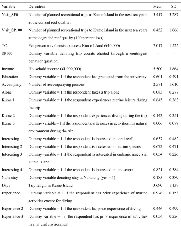
Table 2 Definition of variables used in the model
airport and 2) the airfares for traveling from that airport to the Kumejima airport. First, when respondents used their own car between their house and the nearest airport, the costs were defined as the petrol cost at that time (135 yen), according to the Price Survey of Oil Products, published by the
Variable Definition Mean SD
Visit_SP0 Visit_SP100 TC SP100 Income Education Accompany Alone Kume 1 Kume 2 Kume 3 Interesting 1 Interesting 2 Interesting 3 Interesting 4 Naha stay Days Experience 1 Experience 2 Experience 3
Number of planned recreational trips to Kume Island in the next ten years at the current reef quality;
Number of planned recreational trips to Kume Island in the next ten years at the degraded reef quality (100 percent loss)
Per-person travel costs to access Kume Island (¥10,000)
Dummy variable denoting trip counts elicited through a contingent behavior question
Household income (¥1,000,000)
Dummy variable = 1 if the respondent has graduated from the university Number of accompanying persons
Dummy variable = 1 if the respondent takes a trip alone
Dummy variable = 1 if the respondent experiences marine leisure during the trip
Dummy variable = 1 if the respondent experiences diving during the trip Dummy variable = 1 if the respondent participates in activities in a natural environment during the trip
Dummy variable = 1 if the respondent is interested in coral reef Dummy variable = 1 if the respondent is interested in marine species Dummy variable = 1 if the respondent is interested in endemic insects in Kume Island
Dummy variable = 1 if the respondent is interested in landscape Dummy variable denoting stay at Naha city (yes = 1)
Trip length in Kume Island
Dummy variable = 1 if the respondent has prior experience of marine activities except for diving
Dummy variable = 1 if the respondent has prior experience of diving Dummy variable = 1 if the respondent has prior experience of activities in a natural environment 3.417 0.452 7.017 – 5.500 0.601 2.571 0.083 0.845 0.143 0.006 0.637 0.673 0.054 0.821 0.185 3.690 0.976 0.446 0.054 3.287 1.866 1.525 – 3.864 0.491 1.610 0.277 0.363 0.351 0.077 0.482 0.471 0.226 0.384 0.389 1.137 0.153 0.499 0.226
8
Agency for Natural Resources and Energy (2015).6 For fuel consumption, the average runnable
distance per liter was (26.1 km/L) for passenger cars using petrol, based on the List of Vehicle Fuel Consumption published by the Ministry of Land, Infrastructure, Transport, and Tourism (2015a)7. If
respondents used the highway for time savings, we assumed that they referred to Drive Plaza8 to infer
their costs. The distance from a respondent’s house to the nearest airport was calculated using Google Maps.9 When the respondents used rental cars between their house and the nearest airport, we
estimated the cost as the sum of the price of the rental car and the petrol cost. The rental car fee was calculated using the price list of the nearest rental car shop from a respondent’s house, assuming that the price of a rental car is the one-way car rental fee.10,11 When respondents used taxi services or
public transportation between their house and the nearest airport, the cost was calculated by summing each fee from the appropriate internet site.12,13 Subsequently, airfares from the nearest airport to the
Kumejima airport were calculated using the Airplane Passenger Survey published by the Ministry of Land, Infrastructure, Transport and Tourism (2015b).14 We adopted the discount that most passengers
utilized at each air route. The opportunity cost of time between the respondents’ houses and Kumejima airport was considered to be one-third of the wage rate, following many previous studies.
3. Model estimation
3.1 A PIG model with on-site correction
Let 𝑦! and 𝐱!= (𝑥"!, ⋯ , 𝑥#!)$ denote the number of trips by individual 𝑖 and the 𝑘
-dimensional explanatory variable vector, which includes a constant, respectively. It, then, follows from the exponential mean specification (Cameron and Trivedi, 2013, p. 71) that the conditional mean of 𝑦! is defined as
𝜆! = E(𝑦!|𝐱!) = exp(𝐱!$𝜷) , 𝑖 = 1, ⋯ , 𝑁, (1)
where 𝜷 is the parameter vector. If 𝑦! is independently Poisson distributed with the above mean
parameter 𝜆!, Equation (1) is the well-known standard Poisson regression model. However, this
specification has the so-called equidispersion property, which means that the conditional variance equals its mean. Thus, to relax this restrictive property, we introduce 𝜈!, which expresses the
unobserved heterogeneity of individuals to Equation (1) as follows: 𝜇𝑖 = 𝜆𝑖
𝜈
!,
where 𝜈! is6 Agency for Natural Resources and Energy, 2015. The Price Survey of Oil Products.
http://www.enecho.meti.go.jp/statistics/petroleum_and_lpgas/pl007/results.html#headline4, Accessed date: February 22, 2018.
7 Ministry of Land, Infrastructure, Transport and Tourism., 2015a. The List of Vehicle Fuel Consumption.
http://www.mlit.go.jp/jidosha/jidosha_fr10_000031.html, Accessed date: February 22, 2018.
8 Drive Plaza. http://www.driveplaza.com/dp/SearchTop, Accessed date: February 22, 2018. 9 Google Maps. https://www.google.co.jp/maps, Accessed date: February 21, 2018.
10 Nippon Rent-a-car. https://www.nrgroup-global.com/en/, Accessed date: February 21, 2018. 11 Niconico Rent a car. https://niconicorentacar.jp/, Accessed date: February 21, 2018. 12 TaxiSite. http://www.taxisite.com/ (in Japanese), Accessed date: February 22, 2018.
13 Google Maps Transit. http://maps.google.com/landing/transit/index.html, Accessed date: February 22, 2018. 14 Ministry of Land, Infrastructure, Transport and Tourism., 2015. Airplane Passenger Survey,
9
independent of 𝑦!, and thus E(𝜇!|𝜆!) = 𝜆! because we can assume that E(𝜈!) = 1 without loss of
generality. Thus, unobserved heterogeneity is multiplicatively incorporated into the exponential conditional mean. Now, assuming that 𝑦! follows the Poisson distribution of the mean parameter 𝜇!,
and letting 𝑔(𝜈!) denote the probability density function of 𝜈!, the (marginal) probability density
function of 𝑦!, which is called a mixed Poisson distribution, is shown as
𝑓(𝑦|𝐱) = 9 exp(−𝜆𝜈) (𝜆𝜈) & 𝑦! 𝑔(𝜈)𝑑𝜈 ' ( , (2) where the subscript 𝑖 for an individual is omitted for notational simplicity. This expression is a generalization of the standard Poisson regression model, although specifying 𝑔(𝜈) is necessary to obtain the explicit form of the density. The most popular example is to assume that 𝜈 follows a gamma distribution; that is, the mixed Poisson distribution (2) is the Poisson-gamma mixture, which leads to the well-known negative binomial model.
This study considers the PIG model of Dean et al. (1989), in which 𝜈 follows an inverse Gaussian (IG) distribution. Since E(𝜈) = 1, the probability density function of an IG distribution is given by
𝑔(𝜈) = > 1
2𝜋𝜏𝜈)exp A−
(𝜈 − 1)*
2𝜏𝜈 B,
where Var(𝜈) = 𝜏 > 0 is a shape parameter and unknown. Thus, we have a Poisson-inverse Gaussian mixture as the mixed Poisson distribution (2). From the explicit expression of a PIG distribution shown by Willmot (1987), the conditional probability mass function for the PIG model can be obtained from Equations (3) and (4) below. If y > 0,
ℎ(𝑦|x) =Γ(𝑦 + 1)𝑝(0)𝜆& MΓ(𝑦 − 𝑘)Γ(𝑘 + 1)Γ(𝑦 + 𝑘) N𝜏2O#(1 + 2𝜏𝜆)+&,#* &+" #-( , (3) whereas if 𝑦 = 0, 𝑝(0) = exp N𝜏+"Q1 − √1 + 2𝜏𝜆SO . (4)
Note that as the shape parameter 𝜏 → 0, the PIG model approaches the standard Poisson regression model, and, thus, 𝜏 is the parameter describing overdispersion.
Since the count data are collected via an on-site survey, there are two problems: truncation and endogenous stratification. This problem exists because non-visitors are excluded, which means that the sample is zero-truncated, and visitors who make frequent trips to the site are covered by oversampling. The endogenous stratification problem is one of the particular forms of the so-called choice-based sampling and causes biased and inconsistent estimators of parameters, which may lead to serious mistakes in the statistical inference. Following Shaw (1988), we derive a probability mass
10
function of the PIG model that allows for on-site sampling. Shaw’s correction for the conditional probability density function to control for the effects involved in on-site sampling is given by
ℎ.(𝑦|𝐱) = ℎ(𝑦|𝐱)𝑤(𝑦, 𝜆), 𝑤(𝑦, 𝜆) = 𝑦
E(𝑦|𝐱). (5)
Thus, by applying Equation (5), we can construct a log-likelihood function suitable for the on-site sampling data, as shown in Equation (6):
M log ℎ.(𝑦 !|𝐱!; 𝜽) / !-" = M log ^𝑦! 𝜆!ℎ(𝑦!|𝐱!; 𝜽)_ / !-" = M `log 𝜆! Γ(𝑦!)+ 𝜏 +"Q1 − √1 + 2𝜏𝜆S log aM Γ(𝑦 + 𝑘) Γ(𝑦 − 𝑘)Γ(𝑘 + 1)N 𝜏 2O # (1 + 2𝜏𝜆)+&,#* &+" #-( bc / !-" . (6) Here, 𝜽 = (𝜷$, 𝜏)$ is the unknown parameter. Thus, we obtain the maximum likelihood estimators
based on the PIG model under on-site sampling. 3.2 Expansion to the random effects model
Given that this study aims to measure the recreational benefits, it is necessary to analyze the TCM + CB data. Thus, it is not desirable to analyze each response from a given individual as a univariate count data because ignoring the multivariate dependence will cause an efficiency loss of the estimators and may also affect their consistency. The most natural expansion is to handle it as a multivariate count data, as in Egan and Herriges (2006). However, it is not easy to obtain the estimates because the likelihood function is usually complicated, and its computational burden may be heavy. As an alternative estimation method, their study proposes the use of the seemingly unrelated negative binomial (SUNB) model of Winkelmann (2000) because it avoids computational complexity even though the correlation structure is restrictive. However, Beaumais and Appéré (2010) view multivariate data as a pseudo-panel data. This view implies that the time index of the standard panel data model is regarded as the number of scenarios that accompanies the CB data. Thus, they propose an estimation method invoking the Poisson-gamma random-effects (RE-PGM) model of Hausman et al. (1984), in which each of the random effects is independently and identically distributed as gamma. Following their pseudo-panel approach, we first introduce the random-effects Poisson-inverse Gaussian (RE-PIG) model, which is the expansion of the univariate PIG model. Then, to analyze on-site sampling data, we correct for its sampling effects in a way similar to that given in Section 3.1. Let 𝑦!0 be the number of trips in scenario 𝑗 for individual 𝑖, and let 𝐱!0 = Q𝑥"!0, ⋯ , 𝑥#!0S
$
denote the 𝑘-dimensional explanatory variable vector, including a constant in scenario 𝑗. Similar to Section 3.1, we assume that the conditional mean, which is denoted by 𝜆!0 and satisfies EQ𝜇!0f𝜆!0S =
𝜆!0, can be described as follows:
𝜇!0 = expQ𝐱!0$ 𝜷S 𝜈!, 𝑖 = 1, ⋯ , 𝑁, 𝑗 = 1, ⋯ , 𝐽
11
individuals in a scenario, is considered a random effect that is not dependent on scenario 𝑗; thus, 𝜈!0 = 𝜈!. Hence, although the random effect is denoted by a random variable that follows a common
IG distribution, note that it restricts the correlation structure. The number of trips for each individual is now a multivariate count data; thus, we introduce some new notations: 𝐲! = Q𝑦!", ⋯ , 𝑦!2S$ and
𝐱i! = Q𝐱!", ⋯ , 𝐱!2S$. Then, by expanding Equation (2) in Section 3.1 to the present context, the
conditional probability density function of the RE-PIG model is given by ℎ(𝒚|𝐱i) = 9 kexpQ−𝜇0S 𝜇0 &! 𝑦0! 2 0-" 𝑔(𝜈)𝑑𝜈 ' ( = k 𝜆0&! 𝑦0! 2 0-" 9 exp (−𝜈 ' ( 𝜆2 ∗)𝜈&"∗𝑔(𝜈)𝑑𝜈,
where 𝑦2∗= ∑20-"𝑦0, 𝜆2∗= ∑20-"𝜆0, and the subscript 𝑖 denoting an individual is omitted for
notational simplification. Since 𝑔(𝜈) is the density function of the IG distribution, it follows from the same argument in Section 3.1 that, after some calculation, we obtain the conditional probability mass function for the RE-PIG model as follows:
ℎ(𝒚|𝐱i) = 𝑞(0) M ΓQ𝑦2 ∗+ 𝑘S ΓQ𝑦2∗− 𝑘SΓ(𝑘 + 1) N2𝜏O#Q1 + 2𝜏𝜆2∗S +&" ∗,# * &"∗+" #-( k𝜆0 &! 𝑦0! 2 0-" = 𝑞Q𝑦2∗S k 𝜆0&! 𝑦0! 2 0-" , where 𝑞(0) = exp (𝜏+"(1 − n1 + 2𝜏𝜆 2∗)).
Next, it is necessary to allow for the fact that 𝐲! is assumed to be collected via an on-site survey.
Since there is typically one variable with on-site sampling in 𝐲!, which we set at 𝑦𝑖1
, it is sufficient
to control for the sampling effects only for variable 𝑦1
. Thus, considering this point, the conditional
probability mass function with on-site correction is written asℎ.(𝒚|𝐱i) =𝑞Q𝑦2∗S𝜆"&$+" (𝑦"− 1)! k 𝜆0&! 𝑦0! 2 0-* . (7)
Hence, we can construct a log-likelihood function from Equation (7) in the same way as in Equation (6) in Section 3.1 and obtain the maximum likelihood estimators of parameters, which are given by maximizing ∑ log ℎ.(𝒚
!|𝐱i!; 𝜽) /
!-" with respect to the unknown parameters 𝜽 = (𝜷$, 𝜏)$. Note that
the proposed estimation approach has a similar correlation structure to the SUNB model and the RE-PGM model; thus, the correlation structure among the multivariate count data (that is, the over scenarios) is restricted to be positive and is mainly determined by only one parameter.
3.3 Empirical model
This section introduces our model for empirical analysis, in which dependent variables are constructed from the CB data only; thus, the proposed estimation approach is also capable of dealing with such a case. Following the variable definition from the on-site survey as described in Table 2, the recreational demand function for Kume Island can be specified as:
12
+𝛽7𝐴𝑙𝑜𝑛𝑒!0+ 𝛽8𝐾𝑢𝑚𝑒1!0+ 𝛽9𝐾𝑢𝑚𝑒2!0+ 𝛽:𝐾𝑢𝑚𝑒3!0+ 𝛽"(𝐼𝑛𝑡𝑒𝑟𝑒𝑠𝑡𝑖𝑛𝑔1!0
+𝛽""𝐼𝑛𝑡𝑒𝑟𝑒𝑠𝑡𝑖𝑛𝑔2!0+ 𝛽"*𝐼𝑛𝑡𝑒𝑟𝑒𝑠𝑡𝑖𝑛𝑔3!0+ 𝛽")𝐼𝑛𝑡𝑒𝑟𝑒𝑠𝑡𝑖𝑛𝑔4!0+ 𝛽"5𝑁𝑎ℎ𝑎!0
+𝛽"6𝐷𝑎𝑦𝑠!0+𝛽"7𝐸𝑥𝑝𝑒𝑟𝑖𝑎𝑛𝑐𝑒1!0+ 𝛽"8𝐸𝑥𝑝𝑒𝑟𝑖𝑎𝑛𝑐𝑒2!0+ 𝛽"9𝐸𝑥𝑝𝑒𝑟𝑖𝑎𝑛𝑐𝑒3!0S,
𝑗 = 1, 2, which implies that 𝐱!0=
Q1, 𝑇𝐶!0, 𝑆𝑃100!0, 𝐼𝑛𝑐𝑜𝑚𝑒!0, 𝐸𝑑𝑢𝑐𝑎𝑡𝑖𝑜𝑛!0, 𝐴𝑐𝑐𝑜𝑚𝑝𝑎𝑛𝑦!0, 𝐴𝑙𝑜𝑛𝑒!0, 𝐾𝑢𝑚𝑒1!0, 𝐾𝑢𝑚𝑒2!0,
𝐾𝑢𝑚𝑒3!0, 𝐼𝑛𝑡𝑒𝑟𝑒𝑠𝑡𝑖𝑛𝑔1!0, ⋯ , 𝐼𝑛𝑡𝑒𝑟𝑒𝑠𝑡𝑖𝑛𝑔4!0, 𝑁𝑎ℎ𝑎!0, 𝐷𝑎𝑦𝑠!0, 𝐸𝑥𝑝𝑒𝑟𝑖𝑎𝑛𝑐𝑒1!0, ⋯ , 𝐸𝑥𝑝𝑒𝑟𝑖𝑎𝑛𝑐𝑒3!0S $
and 𝜷 = (𝛽(, 𝛽", ⋯ , 𝛽"9)$ in the framework of Section 3.2. Note that 𝐲!=
(𝑉𝑖𝑠𝑖𝑡_𝑆𝑃0!, 𝑉𝑖𝑠𝑡_𝑆𝑃100!)$ represents the CB data under the hypothetical scenarios, the current reef
condition, and reef extinction (cf. Kragt. et al., 2009). That is, 𝑦" is subject to the on-site correction
because, to collect the data, an on-site survey is employed as mentioned in Section 2.1, and it seems natural that the number of visits will not decrease under the current reef quality. The minimum number of planned trips under the current reef quality is 1 from the on-site survey data. However, 𝑦* indicates
CB data in which the hypothetical scenario of coral reef extinction may lead to a decrease in the number of planned trips.
From the empirical model as specified above, per-person recreational value of a site quality change is measured as
ΔCS =𝜆*− 𝜆"
𝛽" , (8)
where 𝜆* is the number of planned trips associated with a change in reef quality (extinction), 𝜆" is
the number of planned trips under current reef quality, and the coefficient of travel cost is assumed to remain the same after a quality change. In the subsequent section, we compute the estimated ΔCS by replacing 𝜆", 𝜆*, and 𝛽" with their predicted or estimated values 𝜆‹", 𝜆‹*, and 𝛽‹" in Equation (8).
Note that for the predicted number of the trips, 𝜆‹0, the evaluation at the mean of the independent
variables is adopted in the same manner as the previous studies (Whitehead et al., 2000).
4. Estimation results
We estimate the parameters in the recreational demand function constructed in the previous section using two types of econometric approaches: the RE-PGM and RE-PIG models with on-site corrections. Table 3 reports the estimation results for the empirical model using the two approaches. First, the travel cost coefficients (𝑇𝐶), which is our primary interest, are negative, as expected, and significant at the 5% level for both approaches. Moreover, both of the likelihood ratio (LR) statistics reject the null hypothesis that all the coefficients except for the constant are zero at the 1% significance level. Although there are only slight differences in the significance level between the RE-PGM and RE-PIG models, all the coefficients for SP100, Income, Education, Alone, Accompany, Kume, and Interesting 3 are statistically significant at the 10% or lower levels. In particular, the estimates of SP100 support the anticipation that the number of planned trips at the degraded quality will be less
13
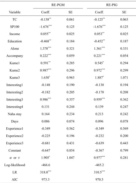
Table 3 Results of RE-PGM and RE-PIG models with on-site correction
RE-PGM RE-PIG
Variable Coeff. SE Coeff. SE
TC -0.138** 0.061 -0.125** 0.063 SP100 -1.676*** 0.125 -1.676*** 0.125 Income 0.055** 0.025 0.053** 0.025 Education -0.468** 0.184 -0.452** 0.187 Alone 1.378*** 0.321 1.361*** 0.331 Accompany 0.222*** 0.059 0.221*** 0.054 Kume1 0.591** 0.285 0.545* 0.294 Kume2 0.987*** 0.296 0.972*** 0.299 Kume3 1.630* 0.963 1.887* 1.071 Interesting1 -0.148 0.190 -0.138 0.194 Interesting2 -0.182 0.205 -0.178 0.208 Interesting3 0.986*** 0.357 0.959*** 0.362 Interesting4 0.131 0.244 0.139 0.247 Naha stay 0.164 0.234 0.213 0.242 Days 0.086 0.074 0.096 0.078 Experience1 -0.349 0.562 -0.349 0.569 Experience2 -0.225 0.196 -0.232 0.200 Experience3 -0.681 0.431 -0.639 0.443 Constant -0.647 0.854 -0.367 0.799 𝛼 or 𝜏 1.905* 1.047 0.977*** 0.281 Log-likelihood -466.6 -465.2 LR 318.0*** 310.5*** AIC 973.3 970.5
Note: ***, **, and * indicate significance at the 1%, 5%, and 10% levels, respectively.
than that at the current quality. Further, the coefficients associated with Kume show statistically positive signs, indicating that the experience of activities during the trip has an increasing effect on future recreational demand. As Days and other dummy variables, except for Interesting 3, are not statistically significant in both approaches, the visitors’ interest in natural resources on Kume Island and past experiences of marine activities did not seem to affect their trip decision-making. Additionally, we find the overdispersion parameters, 𝛼 and 𝜏, to be statistically different from zero at the 10% and
14
1% levels, respectively. This implies that ignoring unobserved heterogeneity will incur efficiency loss of the estimators and may also make them inconsistent. Thus, it seems that the random-effects model approaches with on-site corrections within the framework of pseudo-panel data offer more reliable parameter estimates. Next, to compare the performances of the RE-PGM and RE-PIG models, the Akaike information criterion (AIC; Akaike, 1973) for each approach are reported in Table 3. As the AIC of the RE-PIG model is slightly smaller than that of the RE-PGM model, in addition to the fact that the significance levels of 𝛼 and 𝜏 are largely different from each other, it is conjectured that the former approach is more appropriate for analyzing our on-site sampling data. Thus, the IG distribution would capture overdispersion or unobserved heterogeneity more adequately than the gamma distribution.
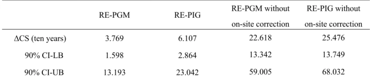
Following Equation (8) and the related discussion in Section 3.3, we can calculate the per-person CS (ΔCS) for ten years, as shown in Table 4, where the 90% confidence intervals of the estimates using the Krinsky-Robb procedure (Haab and MacCnonell, 2002; González-Sepúlveda and Loomis, 2011) are also reported. Notably, Table 4 includes the estimates obtained using the PGM and RE-PIG models while ignoring the on-site sampling issues to examine the effects of on-site corrections. The estimation results of the empirical model corresponding to Table 3 using these approaches are provided in the Appendix. The results show that the annual CS per person trip according to the RE-PGM model (3,796 yen) is smaller than that of the RE-PIG model (6,107 yen). Additionally, although both confidence intervals are asymmetric, the latter has a wider range than the former. We find a similar tendency in both models without on-site corrections. These features seem to reflect the underestimation caused by the inadequacy of the RE-PGM model specification on unobserved heterogeneity, as discussed above. Thus, in terms of the model evaluation, it is preferable to adopt the results of the RE-PIG model in the following discussion. For comparison, Kragt et al. (2009) find the annual CS per person trip to be A$ 83.5, although the per-person recreational value of a site quality change using Equation (8) is not explicitly provided. Thus, by converting Australian dollars into yen using the exchange rate at that time, we find that this amount is approximately 7,097 yen, noting that the hypothetical scenarios (the degraded reef quality) are not the same. Table 4 indicates that CS estimates based on the models without on-site corrections are considerably larger than those of the
Table 4 Estimation results for CS loss
RE-PGM RE-PIG RE-PGM without
on-site correction RE-PIG without on-site correction ΔCS (ten years) 3.769 6.107 22.618 25.476 90% CI-LB 1.598 2.864 13.342 13.749 90% CI-UB 13.193 23.042 59.005 68.032 Unit: ¥10,000
15
corrected models. Given this fact, Kragt et al. (2009) might be overestimating the CS loss because they do not address the on-site sampling issues. Thus, it is crucial to measure recreational values via on-site surveys to control for on-site sampling and adequately specify unobserved heterogeneity or overdispersion.
5. Conclusions
In Japan, coral reefs in Okinawa Prefecture are seriously damaged, and their distributional areas decrease every year. However, there remains a coral reef community in Kume Island that has remarkably high scholarly value. Thus, this study focuses on Kume Island and estimates the recreational demand function using only CB data. Moreover, we propose a PIG model adjusted for an on-site survey and expand it to the random-effects model as an estimation approach. From the empirical analysis, we estimate the CS losses under the hypothetical scenario of current coral reef quality and extinction, finding that the annual CS per person trip is 6,107 yen by the RE-PIG model. To avoid the overestimation of CS, a comparative study suggests that choosing the appropriate estimation approach and the correction for on-site sampling issues is a requirement.
According to a report on the action plan to conserve coral reef ecosystems in Japan for the period 2016–2020, published by the Ministry of the Environment (2015), three priority issues are selected; one of them is the promotion of sustainable tourism in coral reef ecosystems. This report also mentions that coral reef tourism is extremely popular and is an industry that produces the highest economic value in coral reef areas. We find that coral reefs will become increasingly important in terms of the development of the tourism industry on Kuma Island, as conservation of the coral reef ecosystem can enhance its value as a tourism resource. Additionally, on Kume Island, a reproduction project for the protection of coral reefs was initiated in 2019 to promote sustainable activities aimed at recuperation from coral reef bleaching or death. The contents of this project include cultivation, monitoring, and enlightening people on coral reefs. Our results present the necessity of cost-effective policy measures to support such local projects as soon as possible.
Although this study provides valuable input in terms of considering the effects of policy measures that influence the quality of Kume Island’s coral reefs and can be used to assess the recreational benefits of coral reefs in its protection programs, the study has some limitations. First, it is necessary to extend the valuation method to include non-use values to fully consider the total economic value. Second, there is still room for improving the estimation accuracy because the sample size may be small. Third, from a methodological viewpoint, there is a possibility that the PIG model, which controls for on-site sampling, could be extended to latent class or random parameter approaches, as proposed by Hynes and Greene (2013, 2016) based on the negative binomial model. They apply these approaches to a panel dataset of beach users, showing that the unobserved heterogeneity in the framework of their contingent behavior travel cost model can be adequately accounted for even if the
16
data are collected through an on‐site survey. These directions may cover a wide range of specifications on unobserved heterogeneity in pseudo-panel data and would be significant to the field regarding welfare estimation of recreation, which can be a scope for future research.
Acknowledgements
This study was funded by the National Institute for Environmental Studies (NIES) and, also, supported by Japan Society for the Promotion of Science (JSPS), Grant-in-Aid for Young Scientists (B) (Grant Number 17K18038), and the Environment Research and Technology Development Fund (JPMEERF20S11821) of the Environmental Restoration and Conservation Agency of Japan.
17
Appendix
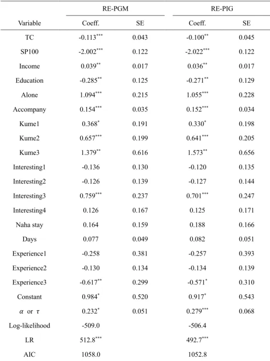
Table A1 Results of RE-PGM and RE-PIG models without on-site correction
RE-PGM RE-PIG
Variable Coeff. SE Coeff. SE
TC -0.113*** 0.043 -0.100** 0.045 SP100 -2.002*** 0.122 -2.022*** 0.122 Income 0.039** 0.017 0.036** 0.017 Education -0.285** 0.125 -0.271** 0.129 Alone 1.094*** 0.215 1.055*** 0.228 Accompany 0.154*** 0.035 0.152*** 0.034 Kume1 0.368* 0.191 0.330* 0.198 Kume2 0.657*** 0.199 0.641*** 0.205 Kume3 1.379** 0.616 1.573** 0.656 Interesting1 -0.136 0.130 -0.120 0.135 Interesting2 -0.126 0.139 -0.127 0.144 Interesting3 0.759*** 0.237 0.701*** 0.247 Interesting4 0.126 0.167 0.125 0.171 Naha stay 0.164 0.159 0.188 0.166 Days 0.077 0.049 0.082 0.051 Experience1 -0.258 0.381 -0.257 0.393 Experience2 -0.130 0.134 -0.134 0.139 Experience3 -0.617** 0.299 -0.571* 0.310 Constant 0.984* 0.520 0.917* 0.543 𝛼 or 𝜏 0.232* 0.051 0.279*** 0.068 Log-likelihood -509.0 -506.4 LR 512.8*** 492.7*** AIC 1058.0 1052.8
18
References
Akaike, H., 1973. Information theory and an extension of the maximum likelihood principle. In Petrov, B.N. and Csaki, F. (eds.), Second International Symposium on Information Theory, pp. 267-281. Akademiai Kiado, Budapest.
Alberini, A., Zanatta, V., and Rosato, P., 2007. Combining actual and contingent behavior to estimate the value of sports fishing in the Lagoon of Venice. Ecol. Econ., 61, 530-541.
Beaumais, O., and G. Appéré., 2010. Recreational shellfish harvesting and health risk: a pseudo-panel approach combining revealed and stated preference data with correction for on-site sampling, Ecol. Econ., 69, 2315-2322.
Bhat, M.G., 2003. Application of non-market valuation to the Florida Keys marine reserve management. J. Environ. Manage., 67, 315-325.
Bockstael, N.E., McConnell, K.E., and Strand, I.E., 1989. Measuring the benefits of improvements in water quality: the Chesapeake Bay. Mar. Resour. Econ., 6, 1-18.
Cabral, R.B., and Geronimo, R.C., 2018. How important are coral reefs to food security in the Philippines? Diving deeper than national aggregates and averages. Mar. Policy., 91, 136-141. Cameron, A.C., and P.K. Trivedi., 2013. Regression analysis of count data, 2nd ed. Cambridge
University Press, New York.
Cesar, H., Burke, L., and Pet-Soede, L., 2003. The economics of worldwide coral reef degradation.
Cesar environmental economics consulting (CEEC).
https://www.wwf.or.jp/activities/lib/pdf_marine/coral-reef/cesardegradationreport100203.pdf, Accessed date: 4 March 2019.
Dean, C., Lawless J.F., and G.E. Willmot., 1989. A mixed Poisson-inverse-Gaussian regression model. Can. J. Stat., 17, 171-181.
Deely, J., Hynes, S., and Curtis, J., 2019. Combining actual and contingent behaviour data to estimate the value of coarse fishing in Ireland. Fish. Res., 215, 53-61.
Egan, K., and Herriges, J., 2006. Multivariate count data regression models with individual panel data from an on-site sample. J. Environ. Econ. Manag., 52, 567-581.
Elliff, C.I., and Kikuchi, R.K., 2017. Ecosystem services provided by coral reefs in a Southwestern Atlantic Archipelago. Ocean Coast. Manage., 136, 49-55.
Englin, J. and Cameron, T.A., 1996. Augmenting travel cost models with contingent behavior data. Environ. Resour. Econ., 7(2), 133-147.
Ferrario, F., Beck, M.W., Storlazzi, C.D., Micheli, F., Shepard, C.C., and Airoldi, L., 2014. The effectiveness of coral reefs for coastal hazard risk reduction and adaptation. Nat. Commun., 5, 3794.
Filippini, M., Greene, W., and Martinez-Cruz, A.L., 2018. Non-market Value of Winter Outdoor Recreation in the Swiss Alps: The Case of Val Bedretto. Environ. Resour. Econ., 71, 729-754.
19
Folkersen, M.V., Fleming, C.M., and Hasan, S., 2018. Deep sea mining's future effects on Fiji's tourism industry: A contingent behaviour study. Mar. Policy, 96, 81-89.
Fujita, Y., and Obuchi, M., 2012. Comanthus kumi, a new shallow-water comatulid (Echinodermata: Crinoidea: Comatulida: Comasteridae) from the Ryukyu Islands, Japan. Zootaxa, 3367(1), 261-268.
González-Sepúlveda, J.M., and Loomis, J.B., 2011. Are benefit transfers using a joint revealed and stated preference model more accurate than revealed and stated preference data alone? In J.C. Whitehead, T.C. Haab, and J.Huang (eds.), Preference Data for Environmental Valuation: Combining Revealed and Stated Approaches, pp.289-302. Routledge, New York.
Guo, J.E, and P.K. Trivedi., 2002. Flexible parametric models for long-tailed patent count distributions, Oxf. Bull. Econ. Stat., 64, 63-82.
Haab, T.C., and McConnell, K.E., 2002. Valuing Environmental and Natural Resources, The Economics of Non-Market Valuation. Edward Elgar, Cheltenham, UK.
Hausman, J.A., Hall, B.H., and Griliches, Z., 1984. Econometric models for count data with an application to the patents-R&D relationship. Econometrica, 52, 909-938.
Hongo, C., and Yamano, H., 2013. Species-specific responses of corals to bleaching events on anthropogenically turbid reefs on Okinawa Island, Japan, over a 15-year period (1995–2009). Plos One, 8, e60952.
Hynes, S., and Greene, W., 2013. A panel travel cost model accounting for endogenous stratification and truncation: A latent class approach. Land. Econ., 89, 177-192.
Hynes, S., and Greene, W., 2016. Preference heterogeneity in contingent behaviour travel cost models with on‐site samples: A random parameter vs. a latent class approach. J. Agr. Econ., 67, 348-367. Intergovernmental Panel on Climate Change (IPCC), 2018. Global warming of 1.5℃, summary for policymakers. https://www.ipcc.ch/sr15/chapter/summary-for-policy-makers/, Accessed date: 4 March 2019.
Kench, P.S., Owen, S.D., and Ford, M.R., 2014. Evidence for coral island formation during rising sea level in the central Pacific Ocean. Geophys. Res. Letters., 41, 820-827.
Kimura, T., Shimoike, K., Suzuki, G., Nakayoshi, I., Shioiri, A., Tabata, A., Tabata, Y., Fujita, Y., Zayasu, Y., Yamano, H., Namizaki, N., Yokoi, K., Ogasawara, K., and Yasumura, S., 2011. Large scale communities of Acropora horrida in the mesophotic zone off Kume Island, Okinawa. J. Jpn. Coral Reef Soc, 13, 43-45 (in Japanese).
Kragt, M.E., Roebeling, P.C., and Ruijs, A., 2009. Effects of Great Barrier Reef degradation on recreational reef-trip demand: a contingent behaviour approach. Aust. J. Agr. Resour. Ec., 53, 213-229.
Lankia, T., and Pouta, E., 2019. Effects of water quality changes on recreation benefits in Finland: Combined travel cost and contingent behavior model. Water Resour. Econ., 25, 2-12.
20
Lienhoop, N., and Ansmann, T., 2011. Valuing water level changes in reservoirs using two stated preference approaches: An exploration of validity. Ecol. Econ., 70, 1250-1258.
Masucci, G. D., Biondi, P., Negro, E., and Reimer, J. D. 2019. After the long summer: Death and survival of coral communities in the shallow waters of Kume island, from the Ryukyu archipelago. Reg. Stud. Mar. Sci., 28, 100578.
Ministry of the Environment. 2015, The action plan to conserve coral reef ecosystems in Japan 2016-2020. Available at: https://www.env.go.jp/nature/biodic/coralreefs/pamph/pamph_full-en.pdf, Accessed date: 4 March 2019.
Morgan, O.A., and Huth, W.L., 2011. Using revealed and stated preference data to estimate the scope and access benefits associated with cave diving. Resour. Energy. Econ., 33, 107-118.
Narukawa, M., and Nohara, K., 2018. Zero-truncated panel Poisson mixture models: Estimating the impact on tourism benefits in Fukushima Prefecture. J. Environ. Manage., 211, 238-246. Oh, S., 2004. Economic Valuation of Okinawa’s Coral Reefs –Economic Analysis of Unavailable
Value by Contingent Valuable Method-, Journal of Business and Economics. Okinawa International University, 32, 35-54 (in Japanese).
Okinawa Prefectural Government, 2018. Ritou Kankei Shiryo (Statistical material about isolated islands) (in Japanese).
https://www.pref.okinawa.jp/site/kikaku/chiikirito/ritoshinko/h31ritoukannkeisiryou.html, Accessed date: 4 March 2019.
Omija, T., Nakasone, K., and Kobayashi, R., 1998. Water pollution caused by soil runoff at a coral reef in Shiraho, Ishigaki Island. Annual Report of the Okinawa Prefectural Institute of Health and Environment, 32, 113-117.
Perry, C.T., Kench, P.S., O’Leary, M.J., Morgan, K.M., and Januchowski-Hartley, F., 2015. Linking reef ecology to island building: Parrotfish identified as major producers of island-building sediment in the Maldives. Geology, 43, 503-506.
Perry, C. T., Kench, P. S., Smithers, S. G., Riegl, B., Yamano, H., and O'Leary, M. J. 2011. Implications of reef ecosystem change for the stability and maintenance of coral reef islands. Glob. Change. Biol., 17(12), 3679-3696.
Prayaga, P., Rolfe, J., and Stoeckl, N., 2010. The value of recreational fishing in the Great Barrier Reef, Australia: a pooled revealed preference and contingent behaviour model. Mar. Policy, 34, 244-251.
Pueyo-Ros, J., Garcia, X., Ribas, A., and Fraguell, R.M., 2018. Ecological restoration of a coastal wetland at a mass tourism destination. Will the recreational value increase or decrease? Ecol. Econ., 148, 1-14.
Robles-Zavala, E., and Reynoso, A.G.C., 2018. The recreational value of coral reefs in the Mexican Pacific. Ocean Coast. Manage., 157, 1-8.
21
Sarker, R., and Surry, Y., 2004. The fast decay process in outdoor recreation activities and the use of alternative count data models. Am. J. Agr. Econ., 86, pp.701-715.
Shaw, D., 1988. On-site samples’ regression problems of non-negative integers, truncation, and endogenous stratification. J. Econometrics., 37, pp.211-223.
Tamura, M., 2006. Toward the Establishment of Strategies for the Sustainable Management of Coral Reefs in Akajima Island; Questioner Survey on Socio-economic Value of Coral Reefs. Midoriishi, 17, 29-33 (in Japanese).
The Cabinet Office in Japan, 2014. Kankyo Mondai ni kansuru Yoron Chosa no Gaiyo (Summary of a public opinion poll about environmental issues) (in Japanese). https://survey.gov-online.go.jp/h26/h26-kankyou/index.html, Accessed date: 22 February 2018.
van Beukering, P., Brander, L., van Zanten, B., Verbrugge, E., and Lems, K., 2011. The economic value of the coral reef ecosystems of the United States Virgin Islands: Final report. IVM Institute for Environmental Studies Report Number: R-11/06., The Netherlands: Amsterdam.
Whitehead, J.C., Haab T.C., and J. Huang., 2000. Measuring recreation benefits of quality improvements with revealed and stated behavior data. Resour. Energy. Econ., 22, 339-354. Willmot, G.E., 1987. The Poisson-Inverse Gaussian distribution as an alternative to the negative
binomial. Scand. Actuar. J. 1987, pp.113-127.
Winkelmann, R., 2000. Seemingly unrelated negative binomial regression. Oxford. B. Econ. Stat., 62, 553-560.
Yamano, H., Satake, K., Inoue, T., Kadoya, T., Hayashi, S., Kinjo, K., Nakajima, D., Oguma, H., Ishiguro, S., Okagawa, A., Suga, S., Horie, T., Nohara, K., Fukayama, N., and Hibiki, A., 2015. An integrated approach to tropical and subtropical island conservation. J. Ecol. Environ., 38(2), 271-279.