Gendered Impacts of Household and Ambient Air
Pollution on Child Health: Evidence from
Household and Satellite-based Data in
Bangladesh
著者
Kurata Masamitsu, Takahashi Kazushi, Hibiki
Akira
journal or
publication title
DSSR Discussion Papers
number
95
page range
1-48
year
2019-01
URL
http://hdl.handle.net/10097/00124285
Data Science and Service Research
Discussion Paper
Discussion Paper No.95
Gendered Impacts of Household and Ambient Air Pollution on Child Health: Evidence from Household and Satellite-based Data in Bangladesh
Masamitsu Kurata, Kazushi Takahashi and Akira Hibiki
January, 2019
Center for Data Science and Service Research Graduate School of Economic and Management Tohoku University
Gendered Impacts of Household and Ambient Air Pollution on Child Health: Evidence from Household and Satellite-based Data in Bangladesh
Masamitsu Kurata ([email protected]), Department of Economics, Sophia University,
Kazushi Takahashi ([email protected]) Department of Economics, Sophia University,
Akira Hibiki ([email protected])
Graduate School of Economics and Management, Tohoku University
Abstract
Reducing health risks from household air pollution (HAP) and ambient air pollution (AAP) is a critical issue in achieving sustainable development worldwide, especially in low-income countries. Children are particularly at high risk because their respiratory and immune systems are not fully developed. Previous studies have identified the adverse impacts of air pollution on child health; however, most have neither focused on HAP and AAP simultaneously nor addressed differences in the timing and magnitude of prenatal and postnatal exposure across genders. This article examines the impacts of prenatal and postnatal exposure to ambient particulate matter with an aerodynamic diameter of 2.5 μm or less (PM2.5) and household use of solid fuels (a main cause of HAP) on child health in Bangladesh. We combine individual-level data from nationally representative surveys with satellite-based high-resolution data on ambient PM2.5. We find that: (1) the use of solid fuels is associated with respiratory illness among girls but not boys; (2) prenatal exposure to ambient PM2.5 adversely affects stunting, without any clear evidence on gender differences; and (3) postnatal exposure consistently increases the risk of both stunting and respiratory illness for both genders. These results provide new evidence on the heterogeneous impacts of AAP and HAP on children in terms of gender and the timing of exposure. The main policy implications are that intervention against HAP would be more effective by targeting girls and that intervention against AAP should cover not only born children but also pregnant mothers. In sum, our findings highlight the importance of protecting women from air pollution and achieving Target 3.9 of the Sustainable Development Goals.
Keywords: Household (indoor) air pollution; Ambient (outdoor) air pollution; child health, child respiratory illness; Bangladesh
1. Introduction
Reducing adverse health impacts from air pollution is one of the most critical global issues. According to Cohen et al. (2017), ambient air pollution (AAP) and household air pollution (HAP) from the use of solid fuels caused 4.2 million and 2.8 million deaths, respectively, in 2015, ranking fifth and tenth in that year’s mortality risk factors. It is also recognized that AAP and HAP have various negative health impacts, such as suppressed visual health and respiratory diseases. Accordingly, reducing the number of deaths and illnesses caused by air pollution has been set as Target 3.9 of the Sustainable Development Goals (SDGs), recognizing the situation as an important agenda for sustainable development (United Nations, 2016).
Children in developing countries are particularly vulnerable due to several biological and socioeconomic factors. First, most poor households in developing countries lack access to modern energy, relying instead on traditional biomass fuels (wood, dung, and agricultural residues), candles, and kerosene for cooking and lighting, all of which intensify HAP (Lam, Smith, Gauthier, & Bates, 2012). Second, rapid economic and population growth is causing AAP to worsen in many developing countries, with enormous particulate matter (PM) caused by agricultural burning, factories, car fumes, and other activities. However, there remain few formal regulations to effectively reduce PM emissions. Third, children in developing countries often need to help their parents
both inside and outside the home. These duties include cooking inside houses without chimneys and open agricultural burning, highly exposing them to toxic HAP and AAP (e.g., Lam et al., 2012). Fourth, since their immune system and lungs are not fully developed, children breathing in air pollutants are more susceptible than adults to HAP and AAP (Schwartz, 2004). Previous studies indicate a significant association between air pollution and infant mortality (Chay & Greenstone, 2003; Jayachandran, 2009), acute lower respiratory infection (Smith & Mehta, 2000), anemia and stunting (Mishra & Retherford, 2006), and low birth weight (Pope et al., 2010). Because damage to health in childhood (or the financial costs of recovery) can have long-term impacts on adult health, economic activities, and well-being (Campbell et al., 2014; Gertler et al., 2014; Baird, Hicks, Kremer, & Miguel, 2016; Miguel & Kremer, 2004), protecting children from both AAP and HAP is an urgent issue to fulfil the SDGs.
Toward that goal, this study aims to identify root causes of the adverse health impacts of air pollution on children aged below five years, such as stunting and respiratory illness. The study focuses on Bangladesh, which is known as one of the world’s most air-polluted countries in terms of AAP; also, most poor households, especially in rural areas, heavily rely on solid fuels for their cooking and lighting, thus worsening HAP (Kudo Shonchoy, & Takahashi, 2017, 2018).
More specifically, this study focuses on several dimensions not extensively studied in the existing literature. First, we elucidate gender differences in the impact of air pollution. Biologically, boys are considered at higher risk than girls due to lower respiratory volumes and narrower peripheral airways in infancy (Clougherty, 2010). However, the direction of gendered bias may not be uniform across different social contexts.1 In Bangladesh, an important traditional norm is the seclusion of women (called
purdah), whereby women must spend long hours inside the home performing household chores (Amin, 1997; Dasgupta,Huq, Khaliquzzaman, Pandey, & Wheeler, 2006). If this also applies to girls, they would be more exposed to and adversely affected by HAP than boys. Second, most previous studies in developing countries, especially south Asia, have focused only on HAP (Pitt, Rosenzweig, & Hassan, 2006; Duflo,Greenstone, & Hanna, 2008; Hanna, Duflo, & Greenstone, 2016; Balietti & Datta, 2017); however, we simultaneously examine HAP and AAP because the latter is becoming a serious problem in Bangladesh. By considering both HAP and AAP, we can specify which channels more seriously damage child health and how these differ between boys and girls. Third,
1 A handful of empirical studies in developed countries show mixed results on gendered impacts: in Stockholm, girls tend to be more affected by outdoor NO2 concentration and use of a gas stove in the home than boys (Pershagen, Rylander, Norberg, Eriksson, & Nordvall, 1995), while, in Germany, boys are more vulnerable to traffic-related air pollution than girls (Gehring et al., 2002).
previous studies reveal that child health is influenced by AAP not only through inhalation but also by transplacental transmission in utero (Sun et al., 2016). Therefore, we calculate the cumulative prenatal exposure to AAP during pregnancy (fixed as 9 months for all children) and postnatal exposure separately for each child. This distinction enables us to disentangle the impacts of exposure to AAP before and after birth. To the best of our knowledge, this is the first study to explore the health impact of both HAP and AAP by considering differences in the timing and magnitude of prenatal and postnatal exposure across genders.
Our empirical analysis is based on individual- and household-level data from a nationally representative survey, combined with satellite-based high-resolution data. Exposure to HAP is measured by a proxy variable on the use of solid fuels (wood, agricultural crops, animal dung, straw, shrubs, grass, and charcoal) using the household data, while exposure to AAP is measured objectively by ambient particulate matter with an aerodynamic diameter of 2.5 μm or less (PM2.5) concentrations using the satellite data. Although it is common to use annual mean or a specific season of PM2.5 for AAP (Dasgupta et al., 2006; Goyal & Canning, 2017), seasonal variation is prominent in Bangladesh. To precisely measure the cumulative pre- and postnatal exposure to PM2.5 for each child, we use an adjusted value of PM2.5 that considers seasonal fluctuations
and children’s birth timing, along with the annual mean of PM2.5. To account for potential endogeneity in the use of solid fuels, we employ not only an ordinary least squares approach but also an instrumental variable approach that uses the share of neighboring households using solid fuels, following an identification strategy suggested by Balietti and Datta (2017).
We find that the use of solid fuels for cooking is associated with respiratory illness in girls but not in boys. Prenatal exposure to ambient PM2.5 adversely affects only stunting, while postnatal exposure increases the risk of both stunting and respiratory illness consistently. These negative effects of AAP (both prenatal and postnatal exposure) are not significantly different between boys and girls. Our findings are robust even after addressing seasonal variations in AAP, potential endogeneity in HAP, and possible selection bias and measurement errors due to migration. These results imply the importance of protecting girls and pregnant mothers to reduce negative health effects from HAP and AAP in our context.
The remainder of this paper is organized as follows. Section 2 briefly overviews the background situation of HAP and AAP in Bangladesh. Section 3 explains details on the conceptual framework, datasets, variables, and empirical framework used in the analysis. In Section 4, we first explain descriptive statistics, then present the results of
regression analysis. Section 5 implements robustness checks and discuss their results. Finally, Section 6 provides concluding remarks with policy implications.
2. Background: Ambient and Household Air Pollution in Bangladesh
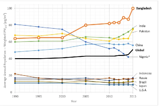
In terms of ambient PM2.5 concentrations, Bangladesh is one of the world’s most air-polluted countries, and its situation continues to deteriorate (Cohen et al. 2017; Wendling, Levy, Esty, de Sherbinin, & Emerson, 2018). As shown in Figure 1, the annual average PM2.5 concentration has increased rapidly since 2000 (Health Effects Institute, 2018a). The main sources of PM2.5 in Bangladesh are agricultural burning, motor vehicles, brick kilns, and smelters, with a large seasonal variation (Begum et al., 2014).
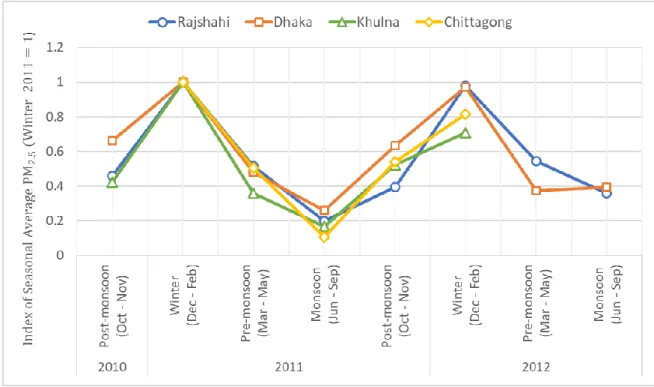
Figure 2 indicates the index of seasonal ambient PM2.5, as measured by air monitoring
stations in four major cities. For all cities, the ambient PM2.5 tends to become acute in the winter, with enormous differences between the winter and monsoon seasons.2
[INSERT FIGURES 1 AND 2 ABOUT HERE]
2 Bangladesh has four seasons: winter (December, January, and February), pre-monsoon (March, April, and May), monsoon (June, July, August, and September), and post-monsoon (October and November).
The Bangladesh government recognizes AAP as a critical environmental issue in the country. In the 7th Five-Year Plan (2016-2020), the government aims to reduce urban PM2.5 from its 2013 level of 78 μg/𝑚3 to 73 μg/𝑚3 in 2020. To achieve this goal, the
government is planning and implementing several programs, such as introducing cleaner fuel and transport standards, and strict enforcement of the Brick Kiln Act 2013 to replace traditional kilns with more efficient Hybrid Hoffman Kilns (Bangladesh Planning Commission, 2016).
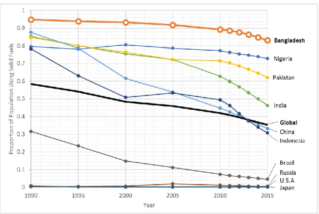
HAP is also serious in the country. In developing countries, the main causes of HAP are domestic activities, such as cooking, heating, and lighting with solid fuels (i.e., biomass fuels or coal). Figure 3 shows that the proportion of the population using solid fuels is higher in Bangladesh than in any of the other 10 most populous countries (Health Effects Institute, 2018a). In 2014, it was reported that 50% of urban households and 95% of rural households used solid fuels for cooking (National Institute of Population Research and Training, Mitra and Associates, & ICF International, 2016).
To mitigate HAP, the government has conducted the nationwide Improved Cook Stove (ICS) program since 2013. If the program is well-executed, ICSs may have a significant impact on reducing HAP (Thomas et al., 2015). The program achieved the dissemination of 1 million ICSs in 2017, although its impacts on HAP have not yet been fully investigated.3
3. Methodology
3.1. Conceptual Framework
In this paper, we investigate the difference in health effects of HAP and AAP between boys and girls. Such differences can be caused by biological differences as sex and social differences as gender (Clougherty, 2010). Biological factors comprise physiologic characteristics (e.g., reproductive organs), body size, and hormonal status, while social factors include cultural norms, roles, and behaviors.4
3 In the neighboring country of India, most ICS programs have failed due to low uptake rates, inappropriate maintenance, and subsequent low usage rates (Hanna et al., 2012; Khandelwal et al., 2017). Regarding ICSs in Bangladesh, Miller and Mobarak (2013) found in field experiments that women have a strong preference for ICSs, but lack decision-making rights on purchases.
4 Although conceptually clear, it is sometimes difficult to distinguish biological and social factors because both can interact with each other (Krieger, 2003).
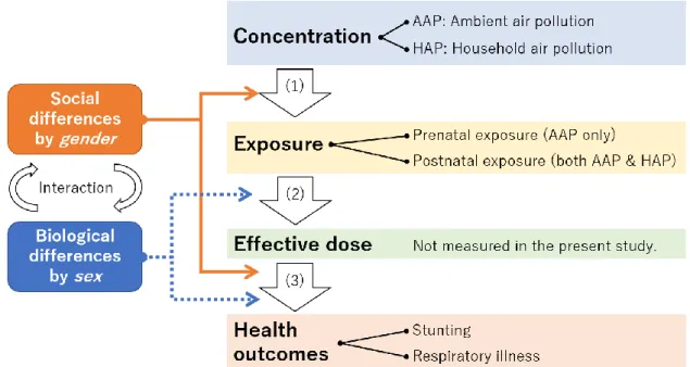
To better understand the differential impacts of biological and social factors on child health, Figure 4 presents our conceptual framework. The overall process is classified into three phases: (1) the first phase from concentration to exposure; (2) the second phase from exposure to effective dose; and (3) the third phase from effective dose to health status (Clougherty, 2010). In the first phase, social factors play an important role, because whether and the extent to which boys and girls are exposed to HAP and AAP depend upon their culture. For example, girls may have higher exposure to HAP if they are expected to help with cooking using solid fuels inside the house, while boys may have higher exposure to AAP if they are expected to help with agricultural work outside the house.
[INSERT FIGURE 4 ABOUT HERE]
Through the second and third phases, biological differences matter because such phases are strongly related to physiological mechanisms. For example, hormonal changes in women during pregnancy can affect toxicant transport throughout the body (Nethery, Brauer & Janssen, 2009). In addition, when children are young (under 5 years old), boys tend to be more vulnerable than girls to air pollution because their respiratory volumes
are lower and peripheral airways are narrower compared to girls (Falagas et al., 2007; Gold et al., 1994).
However, social factors also play a role in the third phase. One of the most crucial differences appears to be gender-biased preferences for seeking health care services. In Bangladesh, women suffering illness have been found to receive health care services significantly less often than men (Ahmed, et al., 2000), whereas opposite results have been reported in other countries (Bertakis, Azari, Helms, Callahan, & Robbins, 2000; Thompson et al., 2016).
Based on the conceptual framework of Figure 4, we ascertain whether the health impacts of HAP and AAP differ between boys and girls. Unfortunately, we cannot examine each phase from (1) to (3) separately, because actual levels of exposure and effective dose are not measured in our study. Instead, we directly estimate the association between concentration of air pollution (HAP and AAP) and health outcomes by controlling biological and social factors.
Since boys are more vulnerable to air pollution in terms of biological characteristics, the negative association between concentration and health outcomes is expected to be stronger for boys than girls. If the opposite result is confirmed, it would suggest that girls are disadvantaged due to social factors.
3.2. Data
This study mainly uses two datasets: the Demographic and Health Survey (DHS) and the Global Annual PM2.5 Grids from MODIS, MISR, and SeaWiFS Aerosol Optical Depth (AOD) with GWR, 1998-2016 (hereafter “the PM2.5 dataset”).
The DHS is a globally standardized survey that collects nationally representative data on population, family planning, and maternal and child health in developing countries (Rutstein & Rojas, 2006). In Bangladesh, the DHS has been conducted eight times since 1993. We use two datasets collected in 2011 and 2014, since both datasets share similar questionnaires and sampling design, with 600 primary sampling units (PSUs) from the whole country. The DHS provides GPS data for each PSU, although the latitude/longitude positions are randomly displaced by up to 2 km in urban clusters and 5 km in rural clusters to protect respondents’ confidentiality. To control for such positional errors, we created a buffer zone around each reported PSU of 2km and 5 km for urban and rural clusters, respectively, and combined the adjusted buffer zone with the PM2.5 dataset.
The PM2.5 dataset (van Donkelaar et al., 2018) contains annual global concentrations of ground-level PM2.5 from 1998 to 2016 at 0.01 degrees (approximately
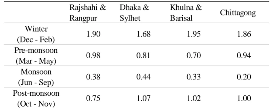
1 km grid), with dust and sea-salt removed. Since this study focuses on the health statuses of children under five years old in the 2011 and 2014 surveys, the PM2.5 dataset from 2005 to 2014 is used. As noted earlier, child health has been found to be affected by AAP not only through inhalation but also by transplacental transmission in utero (Sun et al., 2016); accordingly, we aim to calculate the cumulative prenatal exposure to ambient PM2.5 during pregnancy (fixed as 9 months for all children) and postnatal exposure for each individual child. One drawback of the constructed annual PM2.5 dataset is the lack of seasonal variation in ambient PM2.5. This causes measurement errors in the cumulative exposure to ambient PM2.5 because it gives the same value for all same-aged children, regardless of their actual birth seasons. To more precisely measure cumulative exposure for each child, we adjust annual ambient PM2.5 for each season-specific PM2.5, by setting regional and seasonal parameters of ambient PM2.5 concentrations, and match the adjusted PM2.5 for each child, as shown in Table 1. The parameters are the ratios of the annual mean of ambient PM2.5 based on estimations by Begum et al. (2014). For example, in Rajshahi and Rangpur, exposure to PM2.5 in winter becomes 1.9 times the annual mean, while in the monsoon season it becomes 0.38 times the annual mean. We
logged both cumulative prenatal and postnatal exposure.5
[INSERT TABLE 1 ABOUT HERE]
3.3. Variables
Table 2 indicates the definitions and summary statistics for the outcomes and
covariates used in our analysis. For outcomes, we focus on the health status of children under five years old and examine their stunting and respiratory illness. Stunting (a height-for-age z-score of less than −2) is an objective indicator measured by anthropometry using a height meter. Respiratory illness is measured by coughing and breathing difficulty being reported by the child’s mother in the two weeks before the survey.
[INSERT TABLE 2 ABOUT HERE]
5 In practice, we use log(X+1) where X indicates cumulative prenatal or postnatal exposure to PM2.5, because 1% of the sample (168 children) are less than one month old and their postnatal exposure is assumed to be zero. Although the log(X+1) transformation is widely used in social sciences, some recent papers use the inverse hyperbolic sine (IHS) transformation (e.g., Eyer & Wichman, 2018). We also used IHS transformation, yielding similar results to those of our estimations with the log(X+1) transformation.
As explained in the previous subsection, AAP is measured as the average PM2.5 concentration level within a 2km buffer zone around each urban PSU and a 5km buffer zone around each rural PSU. By contrast, HAP is not measured in numerical values in the DHS: instead, respondents are asked about their main cooking fuel. As a proxy variable for HAP, we use a dummy equal to 1 if a household uses solid fuels (wood, agricultural crops, animal dung, straw, shrubs, grass, and charcoal), and 0 otherwise.
Other covariates are classified into child, parental, and household characteristics, which have been commonly used in the literature. Child characteristics include age, birth order, multiple births, diarrhea symptoms in the two weeks before the survey, and basic vaccination (BCG, measles, and polio) in the past. Birth order and multiple births are known as risk factors for stunting (Jayachandran & Pande, 2017). Incidence of diarrhea symptoms can control for environmental factors unrelated to air pollution that affect child health, such as water pollution.
Mother’s attributes include her age, years of education, body mass index (BMI), relationship with the household head (wife or daughter-in-law), decision-making authority over own health care in the household, and boy preference. Relationship with the household head and authority over health care reflect her social status within the
household, which is strongly connected with exposure to HAP (Pitt et al., 2006). Boy preference is a dummy variable that takes 1 if the mother’s ideal number of boys exceeds the ideal number of girls, and 0 otherwise. This gender-biased preference may affect the mother’s behavior differently for boys against girls. Father’s characteristics comprise his age, years of education, and whether he lives separately from the family.
Household characteristics include the head’s attributes, household composition, religion, cooking location, roof and wall materials, access to electricity, frequency of media use, and household wealth. Cooking outside the house and construction materials with higher permeability can mitigate exposure to HAP but, conversely, promote exposure to AAP, especially in the high dust season (Dasgupta et al., 2006; Dasgupta, Huq, Khaliquzzaman, & Wheeler, 2007). Frequency of media use is a dummy variable that equals 1 if the household takes a newspaper, listens to the radio, or watches TV at least once a week, which should capture exposure to media campaigns for better activities (Madajewicz et al., 2007). For household wealth, we use a set of dummy variables for the wealth index quintile, as calculated by the DHS.
3.4. Empirical Framework 3.4.1. Ordinary least squares
To examine the impact of HAP and AAP on child health in detail, we conduct an individual-level regression analysis using the ordinary least squares (OLS) method, assuming a linear probability model as follows:
where 𝐻𝑒𝑎𝑙𝑡ℎ𝑖ℎd𝑡 is the health outcome for child 𝑖 in household ℎ in district d in
year 𝑡 ; 𝑃𝑀2.5𝑖ℎd𝑡𝑝𝑟𝑒𝑛𝑎𝑡𝑎𝑙 and 𝑃𝑀2.5𝑖ℎd𝑡𝑝𝑜𝑠𝑡𝑛𝑎𝑡𝑎𝑙 are cumulative prenatal and postnatal
exposure levels to ambient PM2.5 concentrations, respectively; 𝑆𝑜𝑙𝑖𝑑ℎd𝑡 is a dummy
variable that equals 1 if a household uses solid fuels for cooking, and 0 otherwise; 𝑿𝑖ℎd𝑡′
is a vector of child attributes, while 𝒁ℎd𝑡′ is a vector of parental and household
characteristics; and 𝜇𝑑, 𝜌𝑡, and 𝜎𝑚 are district, year, and the survey month fixed effects,
respectively. The district fixed effects control any time-invariant regional factors. We also include the survey month fixed effects to control for the survey timing.
Since the DHS is not a panel survey, parameters (α, 𝛽1, 𝛽2, γ, 𝛿, 𝑎𝑛𝑑 𝜃 ) are
pooled estimates using the datasets of 2011 and 2014. The impacts of AAP are measured by 𝛽1 and 𝛽2 , while the impacts of HAP are measured by γ . To examine gender
use sample weights and clustered standard errors at the district level for all regressions.
4. Results
4.1. Descriptive Statistics
Table 3 summarizes the health status of children by year and gender. In 2011,
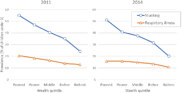
there was no significant differences in stunting and respiratory illness between genders. However, these outcomes for boys became worse than girls in 2014. Figure 5 compares health status by wealth index quintile, confirming the negative correlation between stunting and wealth, although the association is not very clear for respiratory illness.
[INSERT TABLE 3 AND FIGURE 5 ABOUT HERE]
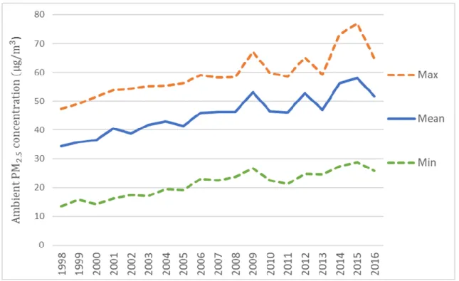
For ambient PM2.5, Figure 6 shows the annual mean, minimum, and maximum values from 1998 to 2016. The annual mean of PM2.5 increased from 34.3 μg/𝑚3 in
1998 to 51.7 μg/𝑚3 in 2016, far exceeding the World Health Organization’s (2015)
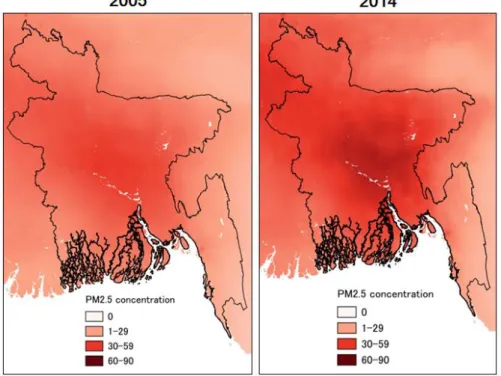
guideline value of 10 μg/𝑚3. However, AAP has not been spread homogeneously over
the whole country. As shown in Figure 7, PM2.5 has increased rapidly in the central, southern, and northeastern regions. The most prominent area is the capital city and its
eastern sub-districts, where PM2.5 has risen more than 15 μg/𝑚3 from 2005 to 2014.
[INSERT FIGURES 6 AND 7 ABOUT HERE]
The main types of cooking fuels are summarized in Table 4. Solid fuels were used by the majority of households, with 87% in 2011 and 85% in 2014. Among them, wood is most prevalent, followed by agricultural crops and animal dung. The composition did not change much during the study period.
[INSERT TABLE 4 ABOUT HERE]
4.2. Regression Analysis 4.2.1. Main results
We first discuss the results of OLS regressions, followed by those of IV in the next section. Table 5 reports the OLS estimation results with and without seasonal variation in ambient PM2.5 (i.e., AAP). There are five main findings .
First, the household’s use of solid fuels for cooking (i.e., HAP) has adverse effects on respiratory illness in girls. The coefficient indicates that the probability of respiratory illness in girls is 4 percentage points higher in households using solid fuels. However, no effects are observed in boys’ respiratory illness or in stunting for either sex. The results are almost the same between estimations with and without seasonal adjustment of PM2.5.
Second, seasonal adjustment substantially influences the coefficients of prenatal exposure to ambient PM2.5. When seasonal variation is not incorporated, the coefficients show that prenatal exposure decreases the risk of respiratory illness in boys and girls (Table 5, columns 3 and 4), which seems counterintuitive. A problem detected in these estimations is high variance inflation factors (VIFs) of prenatal exposure (approximately 7.5 for boys and girls), indicating severe multicollinearity.6
After making seasonal adjustments, the VIFs decrease to acceptable levels (2.9
6 A rule of thumb commonly used is that VIFs exceeding 5 indicate multicollinearity. In the analysis without seasonal variation, there are no other explanatory variables indicating VIFs more than 5, except for prenatal exposure to PM2.5. The mean VIF of all explanatory variables is approximately 2.2 for both boys and girls. In the analysis with seasonal variation, all VIFs are less than 5 and its mean is approximately 2.1 for both boys and girls.
for boys and girls) and the seemingly strange estimated coefficient becomes statistically insignificant with negligible magnitude (Table 5, columns 7 and 8). Therefore, it seems that seasonal variation should be taken into consideration to deal with multicollinearity in prenatal exposure. The results with seasonal adjustment indicate its adverse impact on girls’ stunting, but no effects on respiratory illness.
Third, postnatal exposure to ambient PM2.5 has adverse impacts on all health outcomes for both sexes. With seasonal adjustments, a 1% increase in postnatal exposure increases the probability of stunting by 0.10-0.12 percentage points and that of respiratory illness by 0.01-0.02 percentage points.
Fourth, individual and parental attributes have a reasonable association with child health. As expected, later birth order and multiple births increase the risk of stunting, while diarrhea is strongly related to respiratory illness. Higher maternal BMI and parental education can mitigate stunting, although these effects are weak for respiratory illness. Mother’s decision making on healthcare can reduce risks of stunting and respiratory illness in boys. However, there is no correlation between mother’s boy preference and child health outcomes.
Fifth, among household characteristics, the location of kitchen and house materials have limited impacts on child health. The dummy variable of cooking inside the
house has little effect, even when we include its interaction term with the dummy variable of solid fuels. This is consistent with Pitt et al. (2006). Access to electricity has no significant impacts, perhaps because most households, especially poor ones, are equipped only with low power and low-quality electricity, and so simultaneously use traditional fuels for lighting and cooking. Frequent access to media is associated with a lower probability of respiratory illness in girls. This might be because those households are more likely to be aware of the danger of HAP and AAP for child health.7 Finally,
economic wealth has a stronger association with stunting than respiratory illness, as confirmed in the descriptive statistics. More interestingly, the association between wealth and health is weaker for girls than for boys. In other words, boys’ health is more related to household wealth than that of girls.
4.2.2. Decomposition of Solid Fuel Type
The above analysis uses solid fuels as a single dummy variable. However, different sources of solid fuels may have heterogeneous health impacts (Dasgupta et al.,
7 An alternative explanation is that those households are richer and so able to take better care of their children’s health. However, this explanation seems not convincing as we included wealth classes as control variables.
2006). To examine this possibility, we classify solid fuels by type (firewood, agricultural crops, animal dung, and other biomass), and use each of these four dummies instead of the single dummy variable.
Table 6 shows the results for HAP and AAP with seasonal variation, suppressing
the coefficients of other covariates since they are similar to the previous results in Table
5. We confirm that the use of solid fuels is significantly associated with respiratory illness
only in girls. Three main sources (firewood, agricultural crops, and animal dung) have similar effects on girls’ respiratory illness. The results for AAP are unchanged from the previous results reported in Table 5.
[INSERT TABLE 6 ABOUT HERE]
5. Robustness checks
5.1. Endogeneity in the Use of Solid Fuels
One potential threat to our identification is endogeneity in the use of solid fuels. Although the OLS regression model assumes the use of solid fuels as an exogenous variable, the selection of cooking fuel may not be independent from the error term due to omitted factors affecting both child health and the use of solid fuels. Moreover, there may
be reverse causality: for example, mothers may decide not to use solid fuels because their children have a respiratory illness. Such endogeneity can cause bias in our estimation.
Thus, as a first robustness check, we use the IV approach by exploiting the share of other households using solid fuels in the same PSU as the instrument. A similar instrument is used by Balietti and Datta (2017), who analyze the impact of using solid fuels on stunting in Indian children. The instrument 𝑍ℎ𝑝 for children living in household
ℎ in PSU 𝑝 is defined as:
𝑍ℎ𝑝 =∑𝑘≠ℎ𝑆𝑜𝑙𝑖𝑑𝑘𝑝 𝑁𝑝− 1
where the numerator is the number of households using solid fuels in PSU 𝑝 excluding household ℎ, and 𝑁𝑝 in the denominator is the total number of households minus one
in PSU 𝑝. This instrument is regarded as a proxy variable for the availability of solid fuels, assumed to affect child health only through its impact on the use of solid fuels in household ℎ . In our setting, all outcome variables and the endogenous explanatory variable (use of solid fuels) are dummy variables. Following Angrist and Pischke (2008), we use the standard two-step least squares (2SLS) approach.
regressions. The first-stage result clearly shows that the instrument has a strong and statistically significant effect on the use of solid fuels with sufficiently large F-statistics. Thus, our estimation does not suffer the weak IV problem. It is also confirmed that wealthier households tend to use non-solid fuels for cooking, which is consistent with our expectation.
[INSERT TABLE 7 AROUND HERE]
In the second stage, almost all coefficients of HAP and AAP are qualitatively similar to previous results presented in Table 5. The use of solid fuels has adverse impacts on girls’ respiratory illness. Prenatal exposure to PM2.5 affects stunting in girls, while postnatal exposure affects all outcomes in both sexes. The gender difference in the impacts of wealth on health is also confirmed again. Overall, these results show that our OLS estimations are not sensitive to potential endogeneity concerns.
5.2. Migration
Another possible concern regarding our estimations is migration. While we assume that all children continue to live in the same PSU during pregnancy and after birth,
the living place of some children could change through migration. This raises a potential selection problem, such that ambient PM2.5 cannot be considered exogeneous. Unfortunately, the Bangladesh DHS has no data on migration. However, the Household Income and Expenditure Survey 2016, another nationally representative household survey conducted by the government, reports that only 3% of households experienced any kind of migration within the country (from one district to another) in the last five years from the survey (Bangladesh Bureau of Statistics, 2017). This indirectly supports the view that migration is not a serious problem in our analysis.
To further verify this point, we conducted a sub-sample analysis of children under three years old. Because the probability of migration in the past should be lower for younger children, we can mitigate the possible bias due to migration, if any. Table 8 shows the results of IV estimation for children under three years old. The main findings remain robust: the use of solid fuels affects only girls’ respiratory illness; prenatal exposure to PM2.5 affects stunting for both sexes; and postnatal exposure affects stunting and respiratory illness for both sexes. Again, the impacts of wealth on health outcomes are much smaller for girls.
5. Discussion and Conclusion
This article explores the impacts of household air pollution (HAP) and ambient air pollution (AAP) on child health in Bangladesh, one of the world’s most air-polluted countries. By combining individual-level data from a nationally representative survey and satellite-based high-resolution data on ambient PM2.5 concentrations, we estimated prenatal and postnatal exposure to PM2.5 for each child and examined their adverse impacts on stunting and respiratory illness. The main findings are summarized as follows. First, the use of solid fuels for cooking, a proxy variable for HAP, has adverse impacts on respiratory illness among girls but not boys. Since boys are more vulnerable to air pollution in terms of biological characteristics, these results call attention to social, cultural, and/or behavioral factors. For example, girls may be more susceptible to HAP because they spend longer hours around cooking stoves or receive health care services less frequently than boys (Ahmed, et al., 2000). To assess the plausibility of these explanations, more detailed surveys measuring time use patterns and health-seeking activities by genders are required. These are issues for future research.
Second, prenatal exposure to ambient PM2.5 leads to stunting, while postnatal exposure consistently increases the risk of both stunting and respiratory illness. These
health impacts of AAP are not significantly different between boys and girls. However, the results signify the importance of protecting not only infants but also pregnant mothers from AAP.
Taken together, our results highlight the importance of prioritizing women (girls and pregnant mothers) to reduce the negative impact of air pollution on child health. Although the precise mechanisms that disadvantage girls and pregnant mothers could not be identified in this study, raising awareness of the risk of AAP during pregnancy may be an important policy objective, especially for mothers with lower education levels. Since frequent access to media is found to be negatively associated with girls’ respiratory illness (column 8, Table 5), media campaigns on the risk of HAP may be a possible means to reduce girls’ smoke inhalation. Moreover, the existing program to provide ICSs might be combined with the promotion of risk management practices to further improve child and pregnant mother’s health.
Finally, a potential limitation of our analysis is survival bias, as the mortality rate may be higher in children with more exposure to air pollution. Consequently, our results may underestimate the actual adverse impacts of HAP and AAP on child health, and should be regarded as the minimal level of impact. However, we believe that such bias is not serious in our study as the existing evidence suggests that HAP is not strongly
associated with child mortality in Bangladesh (Naz, Page & Agho, 2015). Because DHS datasets have limited information on stillbirths, further analysis with more detailed child mortality datasets may be useful to investigate the existence and magnitude of survival bias.
References
Ahmed, S. M., Adams, A. M., Chowdhury, M., & Bhuiya, A. (2000). Gender, socioeconomic development and health-seeking behaviour in Bangladesh. Social Science & Medicine, 51(3), 361–371.
Amin, S. (1997). The Poverty–Purdah Trap in Rural Bangladesh: Implications for Women’s Roles in the Family. Development and Change, 28(2), 213–233.
Baird, S., Hicks, J. H., Kremer, M., & Miguel, E. (2016). Worms at work: Long-run impacts of a child health investment. The Quarterly Journal of Economics, 131(4), 1637–1680.
Balietti, A., & Datta, S. (2017). The Impact of Indoor Solid Fuel Use on the Stunting of Indian Children.
Bangladesh Bureau of Statistics (2017). Preliminary Report on Household Income and Expenditure Survey 2016. Dhaka.
Bangladesh Planning Commission (2016). Seventh Five Year Plan FY2016-FY2020: Accelerating Growth, Empowering Citizens. Dhaka.
Begum, B. A., Saroar, G., Nasiruddin, M., Randal, S., Sivertsen, B., & Hopke, P. K. (2014). Particulate Matter and Black Carbon Monitoring at Urban Environment in Bangladesh. Nuclear Science and Applications, 23(1&2).
Bertakis, K. D., Azari, R., Helms, L. J., Callahan, E. J., & Robbins, J. A. (2000). Gender differences in the utilization of health care services. Journal of Family Practice, 49(2), 147–152.
Campbell, F., Conti, G., Heckman, J. J., Moon, S. H., Pinto, R., Pungello, E., & Pan, Y. (2014). Early childhood investments substantially boost adult health. Science, 343(6178), 1478–1485.
Chay K., & Greenstone, M. (2003). The Impact of Air Pollution on Infant Mortality: Evidence from Geographic Variation in Pollution Shocks Induced by a Recession. Quarterly Journal of Economics, 118(3), 1121–1167.
Clougherty, J. E. (2010). A Growing Role for Gender Analysis in Air Pollution Epidemiology. Environmental Health Perspectives, 118(2), 167–176.
Cohen, A. J., Brauer, M., Burnett, R., Anderson, H. R., Frostad, J., Estep, K., ... & Feigin, V. (2017). Estimates and 25-year trends of the global burden of disease attributable to ambient air pollution: an analysis of data from the Global Burden of Diseases Study 2015. Lancet, 389(10082), 1907-1918.
Dasgupta, S., Huq, M., Khaliquzzaman, M., Pandey, K., & Wheeler, D. (2006). Who suffers from indoor air pollution? Evidence from Bangladesh. Health Policy and Planning, 21(6), 444–458.
Dasgupta, S., Huq, M., Khaliquzzaman, M., & Wheeler, D. (2007). Improving Indoor Air Quality for Poor Families: A Controlled Experiment in Bangladesh.
Duflo, E., Greenstone, M., & Hanna, R. (2008). Cooking stoves, indoor air pollution and respiratory health in rural Orissa. Economic and Political Weekly, 71–76.
Eyer, J., & Wichman, C. J. (2018). Does water scarcity shift the electricity generation mix toward fossil fuels? Empirical evidence from the United States. Journal of Environmental Economics and Management, 87, 224–241.
Galliano, A., Ye, C., Su, F., Wang, C., Wang, Y., Liu, C., ... & Steel, A. (2017). Particulate matter adheres to human hair exposed to severe aerial pollution: consequences for certain hair surface properties. International Journal of Cosmetic Science, 39(6), 610–616.
Gertler, P., Heckman, J., Pinto, R., Zanolini, A., Vermeersch, C., Walker, S., ... & Grantham-McGregor, S. (2014). Labor market returns to an early childhood stimulation intervention in Jamaica. Science, 344(6187), 998–1001.
Gordon, S. B., Bruce, N. G., Grigg, J., Hibberd, P. L., Kurmi, O. P., Lam, K. H., … Martin, W. J. (2014). Respiratory risks from household air pollution in low and middle income countries. The Lancet Respiratory Medicine, 2(10), 823–860.
Goyal, N., & Canning, D. (2017). Exposure to Ambient Fine Particulate Air Pollution in Utero as a Risk Factor for Child Stunting in Bangladesh. International Journal of Environmental Research and Public Health, 15(1), 22.
Hanna, R., Duflo, E., & Greenstone, M. (2016). Up in smoke: the influence of household behavior on the long-run impact of improved cooking stoves. American Economic Journal: Economic Policy, 8(1), 80–114.
Health Effects Institute (2018a). State of Global Air 2018. Boston, MA.
Health Effects Institute (2018b). State of Global Air 2018. Special Report. Boston, MA. Jayachandran, S. (2009). Air quality and early-life mortality evidence from Indonesia’s
wildfires. Journal of Human Resources, 44(4), 916-954.
Jayachandran, S., & Pande, R. (2017). Why are Indian children so short? The role of birth order and son preference. American Economic Review, 107(9), 2600-2629.
Khandelwal, M., Hill, M. E., Greenough, P., Anthony, J., Quill, M., Linderman, M., & Udaykumar, H. S. (2017). Why Have Improved Cook-Stove Initiatives in India Failed? World Development, 92, 13–27.
Krieger, N. (2003). Genders, sexes, and health: what are the connections—and why does it matter? International Journal of Epidemiology, 32(4), 652–657.
Kudo, Y., Shonchoy, A. S., & Takahashi, K. (2017). Can solar lanterns improve youth academic performance? Experimental evidence from Bangladesh. The World Bank.
Kudo, Y., Shonchoy, A. S., & Takahashi, K. (2018). Short-term impacts of solar lanterns on child health: experimental evidence from Bangladesh. The Journal of Development Studies, 1–18.
Lam, N. L., Smith, K. R., Gauthier, A., and Bates, M. N. (2012). Kerosene: A review of household uses and their hazards in low and middle-income countries. Journal of Toxicology and Environmental Health, Part B: Critical Reviews, 15(6), 396–432. Lim, S. S., Allen, K., Bhutta, Z. A., Dandona, L., Forouzanfar, M. H., Fullman, N., ... &
Kinfu, Y. (2016). Measuring the health-related Sustainable Development Goals in 188 countries: a baseline analysis from the Global Burden of Disease Study 2015. The Lancet, 388(10053), 1813–1850.
Madajewicz, M., Pfaff, A., van Geen, A., Graziano, J., Hussein, I., Momotaj, H., … Ahsan, H. (2007). Can information alone change behavior? Response to arsenic contamination of groundwater in Bangladesh. Journal of Development Economics, 84(2), 731–754.
Miguel, E., & Kremer, M. (2004). Worms: identifying impacts on education and health in the presence of treatment externalities. Econometrica, 72(1), 159–217.
Miller, G., & Mobarak, A. M. (2013). Gender differences in preferences, intra-household externalities, and low demand for improved cookstoves. National Bureau of Economic Research Working Paper No. 18964.
Mishra, V., & Retherford, R. D. (2006). Does biofuel smoke contribute to anaemia and stunting in early childhood? International Journal of Epidemiology, 36(1), 117–129. National Institute of Population Research and Training, Mitra and Associates, & ICF International (2016). Bangladesh Demographic and Health Survey 2014. Dhaka, Bangladesh, and Rockville, Maryland, USA.
Naz, S., Page, A., & Agho, K. E. (2015). Household air pollution and under-five mortality in Bangladesh (2004–2011). International Journal of Environmental Research and Public Health, 12(10), 12847-12862.
Nethery, E., Brauer, M., & Janssen, P. (2009). Time–activity patterns of pregnant women and changes during the course of pregnancy. Journal of Exposure Science and Environmental Epidemiology, 19(3), 317.
Pitt, M. M., Rosenzweig, M. R., & Hassan, M. N. (2006). Sharing the burden of disease: gender, the household division of labor and the health effects of indoor air pollution in Bangladesh and India. In Stanford Institute for Theoretical Economics Summer Workshop (Vol. 202).
Pershagen, G., Rylander, E., Norberg, S., Eriksson, M., & Nordvall, S. L. (1995). Air Pollution Involving Nitrogen Dioxide Exposure and Wheezing Bronchitis in
Children. International Journal of Epidemiology, 24(6), 1147–1153.
Pope, D. P., Mishra, V., Thompson, L., Siddiqui, A. R., Rehfuess, E. A., Weber, M., & Bruce, N. G. (2010). Risk of low birth weight and stillbirth associated with indoor air pollution from solid fuel use in developing countries. Epidemiologic Reviews, 32(1), 70–81.
Rutstein, S. O., & Rojas, G. (2006). Guide to DHS statistics. Calverton, MD: ORC Macro. Sun, X., Luo, X., Zhao, C., Zhang, B., Tao, J., Yang, Z., ... & Liu, T. (2016). The associations between birth weight and exposure to fine particulate matter (PM2.5) and its chemical constituents during pregnancy: A meta-analysis. Environmental Pollution, 211, 38–47.
Smith, K. R., & Mehta, S. (2003). The burden of disease from indoor air pollution in developing countries: comparison of estimates. International Journal of Hygiene and Environmental Health, 206(4-5), 279-289.
Thomas, E., Wickramasinghe, K., Mendis, S., Roberts, N., & Foster, C. (2015). Improved stove interventions to reduce household air pollution in low and middle income countries: a descriptive systematic review. BMC Public Health, 15(1), 650.
Thompson, A. E., Anisimowicz, Y., Miedema, B., Hogg, W., Wodchis, W. P., & Aubrey-Bassler, K. (2016). The influence of gender and other patient characteristics on health care-seeking behaviour: a QUALICOPC study. BMC Family Practice, 17(1), 38. United Nations (2016). Report of the inter-agency and expert group on sustainable
development goal indicators.
Van Donkelaar, A., Martin, R. V., Brauer, M., Hsu, N. C., Kahn, R. A., Levy, R. C., ... & Winker, D. M. (2016). Global estimates of fine particulate matter using a combined geophysical-statistical method with information from satellites, models, and monitors. Environmental Science & Technology, 50(7), 3762–3772.
Wendling, Z., Levy, M. A., Esty, D. C., de Sherbinin, A., & Emerson, J. W. (2018). The 2018 Environmental Performance Index.
World Health Organization (2005). WHO Air quality guidelines for particulate matter, ozone, nitrogen dioxide and sulfur dioxide. Global Update 2005. Summary of risk assessment.
Figures
Source: Authors’ compilation from Health Effects Institute (2018a).
Note: Data for Nigeria in 2015 (115μg/𝑚3) is excluded from the figure as an outlier due to an ex
tensive dust storm in late 2015 and early 2016 (see Health Effects Institute, 2018b).
Fig 1. Trends in population-weighted annual average 𝐏𝐌𝟐.𝟓 (𝛍𝐠/𝐦𝟑) in the world’s 10 most
Source: Begum et al. (2014)
Source: Authors’ compilation from Health Effects Institute (2018a).
Source: Authors’ compilation based on Clougherty (2010).
Difference in PM2.5 Concentration
Tables
Table 1. Parameters Used as Ratios of Seasonal PM2.5 to Annual Mean.
Note: Authors’ calculations based on Begum et al. (2014).
Rajshahi & Rangpur Dhaka & Sylhet Khulna & Barisal Chittagong Winter (Dec - Feb) 1.90 1.68 1.95 1.86 Pre-monsoon (Mar - May) 0.98 0.81 0.70 0.94 Monsoon (Jun - Sep) 0.38 0.44 0.33 0.20 Post-monsoon (Oct - Nov) 0.75 1.07 1.02 1.00
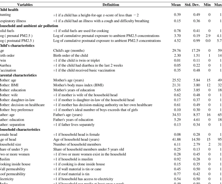
Table 2. Definition and Summary Statistics of Variables
Notes: In addition to the variables in the table, we include in the regression analysis a set of dummy variables for the wealth index quintile (calculated using the DHS), a year fixed effect, district fixed effects, the DHS’s survey month fixed effects.
Variables Definition Mean Std. Dev. Min Max Child health
Stunting =1 if a child has a height-for-age z-score of less than −2 0.39 0.49 0 1
Respiratory illness =1 if a child had an illness with a cough and difficulty breathing 0.15 0.36 0 1
Household and ambient air pollution
Solid fuels =1 if solid fuels are used for cooking 0.78 0.41 0 1
Log ( prenatal PM2.5 ) Log of cumulative prenatal exposure to ambient PM2.5 concentrations 3.70 0.19 2.9 4.1 Log ( postnatal PM2.5 ) Log of cumulative postnatal exposure to ambient PM2.5 concentrations 4.52 0.99 0.0 5.7
Child's characteristics
Age Child's age (months) 29.76 17.29 0 59
Birth order Birth order of the child 2.30 1.51 1 14
Twin =1 if the child is twin or triplet 0.01 0.11 0 1
Diarrhea =1 if the child had diarrhea in the last 2 weeks 0.05 0.22 0 1
Vaccination =1 if the child received basic vaccination 0.35 0.48 0 1
Parental characteristics
Mother: age Mother's age (years) 25.52 5.84 15 49
Mother: BMI Mother's body mass index (BMI) 21.31 3.80 12 32
Mother: education Mother's years of education 5.65 3.85 0 18
Mother: wife =1 if mother is wife of the household head 0.62 0.48 0 1
Mother: daughter-in-law =1 if mother is daughter-in-law of the household head 0.17 0.37 0 1 Mother: decision on healthcare =1 if mother has decision-making authority on her own healthcare 0.61 0.49 0 1 Mother: boy preference =1 if mother's ideal number of boys exceeds that of girls 0.10 0.30 0 1
Father: age Father's age (years) 34.53 8.57 16 65
Father: education Father's years of education 5.29 4.61 0 18
Father: separation =1 if father lives separately 0.13 0.34 0 1
Household characteristics
Female head =1 if household head is female 0.08 0.28 0 1
Age of head Age of household head (years) 41.88 14.50 15 95
Household size Number of household members 6.11 2.79 2 31
Share of under 5 yrs Share of household members under 5 years old 0.25 0.13 0 1
Two or more women =1 if two or more women exist in the household 0.28 0.45 0 1
Muslim =1 if household is muslim 0.92 0.28 0 1
Cooking inside house =1 if cooking is done inside house 0.15 0.35 0 1
Wall permeability =1 if wall material is tin or cane 0.45 0.50 0 1
Roof permeability =1 if roof material is tin 0.77 0.42 0 1
Electricity =1 if household has access to electricity 0.54 0.50 0 1
Table 3. Child Health by Year and Sex (%).
Notes: *** p<0.01; ** p<0.05; * p<0.1.
Boys Girls Difference Boys Girls Difference
(A) (B) (B - A) (C) (D) (D - C)
Stunting 40.3 41.0 0.7 37.6 35.5 -2.0*
Respiratory illness 17.1 16.0 -1.1 15.0 13.2 -1.8**
Table 4. Type of Cooking Fuel
Main type of cooking fuel (%) 2011 2014 Difference
Solid fuels Wood 50.5 54.8 4.3
Agricultural crop 26.0 21.0 -5.0 Animal dung 8.9 7.5 -1.4 Straw/shrubs 1.1 1.0 -0.2 Charcoal 0.2 0.4 0.2 Coal, lignite 0.0 0.3 0.3 Subtotal 86.8 85.0 -1.8 Natural gas 10.7 12.6 1.9 LPG 1.5 1.6 0.1 Biogas 0.3 0.1 -0.1 Electricity 0.2 0.4 0.2 Kerosene 0.2 0.1 -0.1 Other 0.3 0.2 -0.2 Subtotal 13.2 15.0 1.8 Total 100.0 100.0 Non-solid fuels
Table 5. Ordinary Least Squares with and without Seasonal Variation of Ambient PM2.5.
Notes: See Table 2 for other covariates included in regressions. Clustered standard errors at the district level are in parentheses. *** p<0.01; ** p<0.05; * p<0.1.
(1) (2) (3) (4) (5) (6) (7) (8)
Boys Girls Boys Girls Boys Girls Boys Girls
Solid fuel -0.003 0.005 0.009 0.041*** -0.008 0.006 0.010 0.042*** (0.023) (0.024) (0.019) (0.015) (0.023) (0.024) (0.019) (0.015) Log(prenatal PM2.5) 0.214** 0.045 -0.103 -0.127* 0.005 0.111** -0.042 -0.053 (0.090) (0.115) (0.076) (0.074) (0.038) (0.044) (0.034) (0.046) Log(postnatal PM2.5) 0.127*** 0.124*** 0.031*** 0.028*** 0.118*** 0.105*** 0.017** 0.014 (0.015) (0.015) (0.010) (0.009) (0.011) (0.012) (0.009) (0.009) Birth order 0.018*** 0.025*** 0.005 -0.000 0.017** 0.025*** 0.005 0.000 (0.007) (0.008) (0.006) (0.006) (0.007) (0.008) (0.006) (0.006) Twin 0.139** 0.147** -0.009 0.031 0.139** 0.148** -0.006 0.031 (0.058) (0.069) (0.040) (0.040) (0.058) (0.069) (0.039) (0.040) Diarrhea 0.097*** 0.042 0.069** 0.066** 0.094*** 0.040 0.071** 0.068** (0.024) (0.034) (0.031) (0.027) (0.024) (0.035) (0.031) (0.027) Mother: BMI -0.011*** -0.008*** -0.003** -0.001 -0.011*** -0.008*** -0.003** -0.001 (0.002) (0.002) (0.001) (0.002) (0.002) (0.002) (0.001) (0.002) Mother: decision on health -0.025* -0.019 -0.022* -0.006 -0.026* -0.019 -0.022* -0.007
(0.015) (0.013) (0.013) (0.012) (0.015) (0.013) (0.013) (0.012)
Mother: boy preference 0.021 0.042 0.009 -0.003 0.021 0.041 0.010 -0.003
(0.019) (0.027) (0.016) (0.018) (0.019) (0.027) (0.016) (0.018) Mother: education -0.004 -0.007** -0.001 -0.001 -0.004 -0.007** -0.001 -0.001
(0.003) (0.003) (0.002) (0.002) (0.003) (0.003) (0.002) (0.002) Father: education -0.007*** -0.006** -0.001 -0.001 -0.006*** -0.005** -0.001 -0.001
(0.002) (0.002) (0.002) (0.001) (0.002) (0.002) (0.002) (0.001)
Cooking inside house 0.019 0.024 0.006 -0.007 0.018 0.023 0.005 -0.006
(0.021) (0.018) (0.015) (0.014) (0.020) (0.018) (0.015) (0.014) Wall permeability 0.018 0.021 -0.025 0.002 0.022 0.020 -0.025 0.001 (0.019) (0.022) (0.016) (0.015) (0.018) (0.022) (0.016) (0.015) Roof permeability -0.041* 0.013 0.027 -0.007 -0.038* 0.012 0.027 -0.008 (0.021) (0.022) (0.016) (0.012) (0.021) (0.021) (0.016) (0.012) Access to electricity 0.011 0.019 0.010 0.003 0.010 0.020 0.011 0.003 (0.027) (0.019) (0.013) (0.015) (0.027) (0.019) (0.014) (0.015) Access to media -0.005 0.004 -0.006 -0.026** -0.006 0.004 -0.007 -0.026** (0.019) (0.018) (0.014) (0.012) (0.018) (0.018) (0.014) (0.012) Wealth quintile: poorer -0.062** -0.006 -0.030* -0.002 -0.061** -0.008 -0.031* -0.002
(0.028) (0.019) (0.017) (0.018) (0.029) (0.019) (0.017) (0.018) Wealth quintile: middle -0.081*** -0.044* -0.033 -0.007 -0.080*** -0.045* -0.034 -0.008
(0.029) (0.023) (0.022) (0.018) (0.029) (0.023) (0.022) (0.018) Wealth quintile: richer -0.128*** -0.073*** -0.048* -0.020 -0.126*** -0.076*** -0.050* -0.020
(0.032) (0.027) (0.026) (0.024) (0.032) (0.027) (0.026) (0.024) Wealth quintile: richest -0.214*** -0.160*** -0.064** -0.008 -0.208*** -0.162*** -0.065** -0.009
(0.043) (0.035) (0.027) (0.030) (0.043) (0.035) (0.027) (0.030)
Other control variables Yes Yes Yes Yes Yes Yes Yes Yes
District fixed effects Yes Yes Yes Yes Yes Yes Yes Yes
Survey month fixed effects Yes Yes Yes Yes Yes Yes Yes Yes
Observations 7470 7124 8094 7672 7470 7124 8094 7672
Adjusted R-squares 0.106 0.122 0.038 0.030 0.107 0.123 0.038 0.029
Without seasonal variation With seasonal variation
Table 6. Ordinary Least Squares with Seasonal Variation in Ambient PM2.5: Health Effects of Household Air Pollution by Solid Fuel Type.
Notes: See Table 2 for other covariates included in regressions. Clustered standard errors at the district level are in parentheses. *** p<0.01; ** p<0.05; * p<0.1.
(1) (2) (3) (4)
Boys Girls Boys Girls
Solid fuel: firewood -0.008 0.008 0.007 0.041*** (0.023) (0.024) (0.018) (0.015) Solid fuel: agri. crop -0.011 -0.006 0.007 0.054*** (0.029) (0.029) (0.025) (0.017) Solid fuel: animal dung -0.007 0.021 0.009 0.068*** (0.039) (0.040) (0.027) (0.024) Solid fuel: others -0.011 -0.005 0.098 -0.005
(0.079) (0.079) (0.093) (0.043) Log(prenatal PM2.5) 0.005 0.112** -0.041 -0.054
(0.038) (0.044) (0.035) (0.046) Log(postnatal PM2.5) 0.118*** 0.106*** 0.018** 0.014
(0.011) (0.012) (0.009) (0.009)
Other control variables Yes Yes Yes Yes
District fixed effects Yes Yes Yes Yes
Survey month fixed effects Yes Yes Yes Yes
Observations 7470 7124 8094 7672
Adjusted R-squares 0.106 0.123 0.038 0.029 Stunting Respiratory illness
Table 7. Instrumental Variable Estimation with Seasonal Variation in Ambient PM2.5: Children under Five Years Old.
Notes: See Table 2 for other covariates included in regressions. Clustered standard errors at the district level are in parentheses. *** p<0.01; ** p<0.05; * p<0.1.
(1) (2) (3) (4) (5) (6)
Boys Girls Boys Girls Boys Girls
Share of solid fuel in PSU 0.779*** 0.814*** (0.023) (0.020) Solid fuel 0.020 0.008 0.003 0.054** (0.053) (0.057) (0.041) (0.024) Log(prenatal PM2.5) -0.044** -0.025 0.008 0.111*** -0.043 -0.052 (0.019) (0.020) (0.036) (0.043) (0.034) (0.044) Log(postnatal PM2.5) 0.015*** 0.006 0.117*** 0.105*** 0.018** 0.014* (0.004) (0.006) (0.011) (0.012) (0.008) (0.009) Wealth quintile: poorer -0.020** -0.018** -0.060** -0.007 -0.031* -0.002
(0.008) (0.007) (0.028) (0.019) (0.017) (0.018) Wealth quintile: middle -0.036** -0.044*** -0.079*** -0.045* -0.034 -0.007
(0.014) (0.010) (0.029) (0.023) (0.022) (0.018) Wealth quintile: richer -0.041** -0.054*** -0.123*** -0.075*** -0.050** -0.019
(0.019) (0.015) (0.032) (0.025) (0.025) (0.024) Wealth quintile: richest -0.015 -0.032 -0.204*** -0.162*** -0.066** -0.006
(0.030) (0.026) (0.041) (0.035) (0.028) (0.030)
Other control variables Yes Yes Yes Yes Yes Yes
District fixed effects Yes Yes Yes Yes Yes Yes
Survey month fixed effects Yes Yes Yes Yes Yes Yes
Observations 8094 7672 7470 7124 8094 7672
Adjusted R-squares 0.740 0.752 0.106 0.123 0.038 0.029 First stage F-statistics 24811.2*** 3234.0***
First stage
Solid fuel Stunting Respiratory illness Second stage
Table 8. Instrumental Variable Estimation with Seasonal Variation in Ambient PM2.5: Children under Three Years Old.
Notes: See Table 2 for other covariates included in regressions. Clustered standard errors at the district level are in parentheses. *** p<0.01; ** p<0.05; * p<0.1
(1) (2) (3) (4) (5) (6)
Boys Girls Boys Girls Boys Girls
Share of solid fuel in PSU 0.770*** 0.814*** (0.020) (0.024) Solid fuel -0.057 -0.013 0.008 0.083** (0.070) (0.066) (0.047) (0.033) Log(prenatal PM2.5) -0.062*** -0.009 0.132*** 0.122** -0.048 -0.074 (0.023) (0.025) (0.047) (0.055) (0.041) (0.045) Log(postnatal PM2.5) 0.012* 0.004 0.059*** 0.052*** 0.043*** 0.017 (0.006) (0.007) (0.016) (0.014) (0.011) (0.012) Wealth quintile: poorer -0.018 -0.020** -0.067* 0.004 -0.048** -0.014
(0.012) (0.010) (0.037) (0.023) (0.024) (0.025) Wealth quintile: middle -0.028 -0.046*** -0.069** -0.008 -0.070** -0.034
(0.020) (0.014) (0.028) (0.031) (0.029) (0.023) Wealth quintile: richer -0.027 -0.051*** -0.107*** -0.044 -0.074** -0.045
(0.023) (0.017) (0.034) (0.032) (0.035) (0.027) Wealth quintile: richest 0.021 -0.039 -0.162*** -0.138*** -0.097*** -0.040
(0.038) (0.032) (0.042) (0.046) (0.034) (0.035)
Other control variables Yes Yes Yes Yes Yes Yes
District fixed effects Yes Yes Yes Yes Yes Yes
Survey month fixed effects Yes Yes Yes Yes Yes Yes
Observations 4721 4547 4354 4205 4721 4547
Adjusted R-squares 0.740 0.760 0.133 0.122 0.034 0.029 First stage F-statistics 2476.1*** 21800.2***
First stage
Solid fuel Stunting Respiratory illness Second stage