Analysis using Adaptive Tree Structured Clustering
Method for Medical Data of Patients
with Coronary Heart Disease
Takashi Yamaguchi*
1, Takumi Ichimura*
2, and Kenneth J. Mackin*
1 1) Tokyo University of Information Sciences, Department of Information Systems4-1Onaridai, Wakaba-ku, Chiba, 265-8501 Japan email: [email protected]
2) Hiroshima City University, Graduate School of Information Sciences 3-4-1 Ozuka-Higashi, Asa-Minami-ku, Hiroshima, 731-3194, Japan
email: [email protected]
Abstract—It is known that the classification of medical data is
difficult problem because the medical data has ambiguous information or missing data. As a result, the classification method that can handle ambiguous information or missing data is necessity. In this paper we proposed an adaptive tree structure clustering method in order to clarify clustering result of self-organizing feature maps. For the evaluating effectiveness of proposed clustering method for the data set with ambiguous information, we applied an adaptive tree structured clustering method for classification of coronary heart disease database. Through the computer simulation we showed that the proposed clustering method was effective for the ambiguous data set.
I. INTRODUCTION
Self-organizing feature map (SOM) is a type of artificial neural network proposed by T.Kohonen[1]. SOM is trained using unsupervised learning to produce low dimensional representation of the training samples while preserving the topological information of the input space. SOM has been applied to wide range of complex problems, such as speech recognition, optimal character recognition, text classification, etc. However, in the viewpoint of clustering algorithm, the clustering result of SOM depends on visual human decision. The boundary of cluster is not clear.
In this paper we propose an adaptive tree structure clustering method in order to clarify clustering result of SOM. Tree structured SOM has been previously proposed[2]. The tree structured SOM has a tree node as the competitive layer unit. On the other hand our proposed tree structured method has tree nodes to distinguish the clusters such as C4.5[3]
The proposed clustering method recursively divides the data set to 2 subsets based on SOM and hierarchical clustering. As a result our clustering method obtains the appropriate number of clusters and the tree structure that shows potential hierarchical relationship in data. In the previous research, we applied the proposed clustering method for the classification of iris data[4]. From the experimental results by using iris data set, we confirm our clustering method can extract the tree structure without decreasing SOM classification performance.
The clustering method is expected to be effective for application to complex data sets including ambiguous information such as medical data. It is known that the classification of medical data is difficult problem because the database developed from the clinical record includes ambiguous information or missing data such as biochemical test. When the medical data set is classified based on the feature of each record such as clustering algorithm, it is necessary to handle the ambiguousness of record.
In this paper, we applied an adaptive tree structured clustering method for classification of coronary heart disease database developed by Suka et al[5]. Finally we report the computer simulation result of proposed clustering method.
II. CLUSTERING METHOD
A. Clustering Algorithm
Clustering is a type of unsupervised classification which divides the data set into some number of subsets based on distance between each data. The clustering algorithms can be classified to hierarchical clustering and the non-hierarchical clustering.
In the hierarchical clustering algorithm, there are 2 different approaches: the agglomerative and the divisive. The agglomerative hierarchical clustering algorithms are more popular and known as cluster analysis in the field of statistics. Generally hierarchical clustering indicates the agglomerative hierarchical clustering. The agglomerative clustering start with each element as a separate cluster, and recursively merge clusters until the number of clusters equals given number. The divisive hierarchical clustering algorithm is composed by combination of agglomerative hierarchical clustering or non-hierarchical clustering. The divisive clustering start with a single cluster combining all the elements and recursively divide the cluster to some number of the clusters.
Typical agglomerative hierarchical clustering algorithms are single linkage method, group average method and Ward’s method. K-means[6] and SOM are non-hierarchical clustering
Fourth International Workshop on Computational Intelligence & Applications
algorithms. The proposed adaptive tree structured clustering is a type of the divisive hierarchical clustering algorithm that combining agglomerative hierarchical clustering algorithm and non-hierarchical clustering algorithm.
B. Hierarchical Clustering Algorithm
When the data set S is a set of n dimensional real vectors xi
= (xi1 xi2 … xin), S = {xi}, i = 1,…, N and let a family of disjoint
subsets of S at the clustering time step tc be a(tc) = {ak(tc) | ak(tc) ∊
S, ak(tc) ≠ φ, ∪a(tc) = S, ak(tc) ∩ ak’(tc) = φ,}, k, k’ = 1,…, |a(tc)|, k
≠ k’, where ak(tc) call kth cluster at the clustering time step tc,
the element of ak(tc) be xki, ki = 1,…,kn, xki ∊ S, the
agglomerative hierarchical clustering algorithm is described as follows.
The agglomerative hierarchical clustering algorithm start with each element as separate cluster, such that ak(0) = {xki},
ki=1. |a(tc)| = N. The agglomerative hierarchical clustering algorithm repeats following 3 steps: selecting clusters, merging clusters and updating distance, until the number of cluster |a(tc)| equals to 1. In the step of selecting clusters, the pth and qth cluster that minimizes distance function d(ap(tc), aq(tc)) is
selected where p, q = 1,…, |a(tc)| , p ≠ q. The distance function
d(ap(tc), aq(tc)) is difference between each method.
Next, in the step of merging cluster, the selected pth and qth cluster are merged to new cluster ap(tc) ∪ aq(tc). The new cluster
ap(tc) ∪ aq(tc) is used instead of cluster ap(tc) and aq(tc) in the next
time step tc + 1. In the step of updating distance, the distances between each cluster are re-calculate based on set of cluster
aq(tc+1) at next time tc + 1. The computational complexity of the
agglomerative hierarchical clustering algorithm is O(N2) by using Lance-Williams update formula[7] for the update distance. Lance-Williams update formula is defined as follow:
( )
,
( ) ( ))
(
( ),
( ))
(
( ),
( ))
(
1 1 2 tc q tc r tc p tc r tc q tc p tc ra
a
d
a
a
d
a
a
a
d
+∪
=
α
⋅
+
α
⋅
( ),
( ))
(
(
( ),
( ))
(
( ),
( ))
)
(
tc q tc r tc p tc r tc q tc pa
d
a
a
d
a
a
a
d
+
⋅
−
⋅
+
β
γ
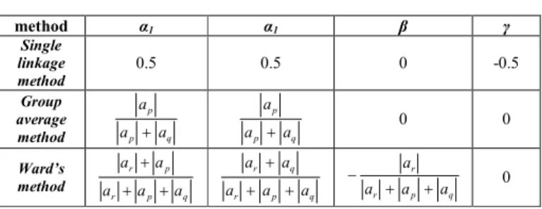
(1)where r = 1,…, |a(tc)|, r ≠ p, q; and α1, α2, β and γ are
coefficients of each agglomerative hierarchical clustering method defined as table I.
The divisive hierarchical clustering algorithm is recursively take the procedure of the partitioned hierarchical clustering algorithm. The divisive hierarchical clustering algorithm described as follows.
The divisive hierarchical clustering algorithm start with a cluster includes whole element of input data set such that a(0) =
S. At the time step tc, The divisive hierarchical clustering
algorithm recursively divide the each or selected cluster ak(tc) to
K new cluster Ak(tc) = {Akl(tc) | Akl(tc) ∊ S, Akl(tc) ≠ φ, ∪Ak(tc) = ak,
Akl(tc) ∩ akl’(tc) = φ,}, l, l’ = 1,…, K, l ≠ l’, where K is the given
number. At the time step tc + 1, the new clusters Akl(tc) is used
instead of divided cluster ak(tc). The criteria to select the divided
cluster and terminate the recursive procedure depend on each method divisive hierarchical clustering algorithm.
TABLE I. PARAMETER OF LANCE WILLIAMS UPDATE FUNCTION
method α1 α1 β γ Single linkage method 0.5 0.5 0 -0.5 Group average method p q p a a a + p q p a a a + 0 0 Ward’s method q p r p r a a a a a + + + q p r q r a a a a a + + + q p r r a a a a + + − 0
III. ADAPTIVE TREE STRUCTURED CLUSTERING METHOD
The proposed adaptive tree structured clustering algorithm is the dividing hierarchical clustering algorithm that composed with SOM and agglomerative hierarchical clustering algorithm. The proposed clustering method recursively divide the selected cluster ak(tc) to K = 2 new cluster Akl(tc) based on the
result of SOM that training using data subset ak(tc).The criterion
to select the divided cluster is defined by the decreasing of means square error of ak(tc) and Akl(tc). The criterion to terminate
the recursive procedure is that each cluster ak(tc) do not satisfied
criterion to select the divided cluster. These process can be considered to the Kary tree generation process – the cluster
Akl(tc) is node, tc is depth of the tree. In other word the proposed
method start with only root node and recursively create K node. The node creation depends on the clustering result in each node. The each node has data subset of parent node data subset. As a result a number of cluster and a tree structure are obtained.
In each node of the tree structure there are the following 4 steps: (1) SOM training, (2) re-clustering (3) clustering, (4) node generation. The criterion for the end of the SOM training and the retraining in the re-clustering step are determined from the error between input vector and weight vector. This is discussed at the end of this section because the criteria are interdependent on both the error of parent node and the classified 2 child nodes
A. Step of SOM training
The step of SOM training is based on online training algorithm of basic SOM. Let the input data set be S, and the weights of the competitive layer where the units are arranged into a 2 dimensional lattice be the set of n dimensional real vectors W = {wj}, j = 1,…, jmax, wj = (wj1 wj2 … wjn). The
value of weight vectors wj is initialized using by random values.
In the SOM training, while repeating the steps of determining the winner unit and updating the weight vector for the selected input vector, the weight vector values converges towards the input vector values.
At the each training time step t = 1,…, tmax, the winner unit c that minimizes the distance between input vector xi(t)
and jth weight vector wj(t) is selected When Euclidean distance
is used, the winner unit c is determined by equation (2)
{
(
)
(
)
}
min
arg
t
t
c
i j jx
−
w
=
(2)For the updating of the weight vectors, the weight vectors of the winner unit and its neighbors on the competitive layer are updated. The weight modification defined as follows:
(
(
)
(
)
)
)
(
)
1
(
t
h
cjt
it
jt
jx
w
w
+
=
⋅
−
∆
(3)where hcj(t) is the neighborhood function. The Gaussian type
neighborhood function is defined as follows:
−
−
⋅
=
)
(
2
exp
)
(
2 2t
r
r
t
h
cj c jσ
λ
(4)where λ(t) is learning-rate factor, || rj - rc || is distance between
winner unit c and unit j in coordinates of the competitive layer,
σ2(t) is a parameter that define the width of updating. λ(t) and
σ2(t) are monotonic decreasing parameters for training step t. In this paper we used following function for λ(t) and σ2(t):
( )
( )
tt
λ
λ
λ
=
0
⋅
′
(5)( )
( )
tH
H
t
σ
σ
σ
=
+
(
0
−
)
⋅
′
(6)where λ’ (0 < λ’ < 1.0) and σ’ (0 < σ’ < 1.0) are parameters, and H defines minimal width of kernel. SOM approximates set of input vectors S by set of weight vectors W, and visualizes the relation between the vectors in the input S through the neighborhood learning.
B. Step of Clustering
After the SOM training, input space S is divided into 2 subsets Ak based on the SOM training result. When the SOM
training converges, winner unit c and units that have close weight vector values with weight vector values of the winner unit c, forms a Voronoi cell on the map. The relative location of the winner units on the map shows the relationship between the input vectors. Therefore clustering using SOM can be decided by the weight vector values and neighbor information of each winner unit.
When the set of winner units is C = { wci }, ci = 1,…, cimax
and the set of disjoint subset of C is b = {bkc | bkc ∊ C, bkc ≠ φ,
∪b = C, bkc ∩ bkc’ = φ,}, kc, kc’ = 1,…, |b|, kc ≠ kc’; the C is
recursively merged using agglomerative hierarchical clustering algorithm until .|bkc| = k. 2 subset Ak is obtained from equation
(2) and bkc where kc=k. In the process of merging winner units,
when the set of winner units in the neighbor of winner unit ci is
Nci, the cpth and cqth merged winner unit satisfies expression
(4) where cp, cq = 1,…, cimax, cp ≠ cq.
cq
cp
N
cq
∈
cp,
≠
(7)For distance function d(bkp, bkq), we use following equation
(6) based on group average method.
cq cp a a kq p k kq cq kp cp
a
a
d
w
w
w w−
=
∈ ∈min
,)
,
(
(8)C. Node Generation and SOM training Termination
When the decreasing of the quantization error is large, 2 new child nodes are created. Let the quantization error of data subset be E(A), the quantization error of cluster before division be E(A1∪ A2), and the quantization error of clusters after
division be E(A1) and E(A2). 2 new child nodes are created
which satisfy expression (7):
(
A
A
)
E
( )
A
E
( )
A
( )
D
E
1∪
2−
1−
2>
θ
(9)( )
∑
∈−
=
k p A k p k kA
E
ww
w
(10)where wk is centroid of Ak and θ(D) is threshold for node
creation that is monotonic decreases function. In this paper we used following function for θ(D):
( )
( )
Dk
k
D
θ
θ
θ
=
0
⋅
′
(11)where θ(0) is initial value of node creation threshold and
θ’(0<θ’<1) is the decreasing rate of node creation threshold.
The child nodes have separate SOMs trained with the corresponding subset. Let parent node be Nodeb, child nodes be
Nodeb = {Nodekb}, k=1,2, SOM of parent node is SOMb, and
SOM of child nodes are SOMb = {SOMkb}, k = 1, 2. The parent
node Nodeb divide the data set S to the subsets Ak from the
result of SOMb with data set S. The new child nodes Nodekb
divide the data subsets Ak from the result of SOMkb
At the training step t of the SOMkb, let ek be the error
between input vector xik and weight vector wcik of the
corresponding winner unit ci. The learning error ek is show as equation (12).
∑
=−
=
max 1)
(
i i k ci k i kt
e
x
w
(12)The average change in learning error between training step t to t + τ calculate by equation (13):
∫
+ ∆→∆
∆
−
−
=
∆
t τ t k k t kdt
t
t
t
e
t
e
t
e
(
)
lim
(
)
(
)
0 (13)where ∆t is the length of training steps to sample the learning error ek(t), and τ defines the length of training steps to calculate average. For the average change in learning error ∆ek, we considered approximate equation (14) because of the calculation cost of ek and ∆ek is very high.
dt
t
t
t
e
t
e
t
e
t t k k k∫
+−
∆
−
∆
=
∆
(
)
τ(
)
(
)
,(
∆t
<
τ
)
(14)When ∆e is calculated by equation (15), The training of
SOMkb ends when expression (16) or (17) is satisfied:
2 1
e
e
e
=
+
∆
(15)( )
D
e
<
ϕ
∆
(16)( )
D
e
k<
ϕ
k∆
(17)where D is the number of the tree depth, φ(D) and φk(D) are
thresholds of the end criterion that is a monotonic decreasing function. In this paper we used following function for φk(D):
( )
( )
Dk
k
D
ϕ
ϕ
ϕ
=
0
⋅
′
(18)where φk(0) is initial value of node creation threshold and
φ’(0<φ’<1) is the decreasing rate of node creation threshold. D. Step of Re-Clustering
Let the training step when the end criterion is satisfied be T. In the end of the clustering step, it is necessary to satisfy equation (19)
A
A
t tˆ
lim
()=
∞ → (19)However, SOM training has the problem that the result is different dependant on the weight initialization and the order of training input. In prior experiments the problem that the class boundary is not constantly decided was confirmed by using a data sets in which the data exist near the class boundary.
For resolving this problem, data set S is re-clustered by checking the error of each child node’s SOMs. The error eik
between input vector xik and weight vector wcik of
corresponding winner node ci is expressed as equation (20).
k ci k i k i
e
=
x
−
w
(20)The error ei¬k between input vector xik and weight vector
wci¬ k of corresponding winner unit ci is described by the
following. k ci k i k i
e
¬=
x
−
w
¬ (21)If expression (22) is satisfied then xik is removed from the
current subset Ak and added to subset A¬k:
ς
>
k ie
, k i k ie
e
>
¬ (22)where ς is the threshold for re-clustering. After S is re-clustered,
SOMkb is retrained. For the retraining of SOM, an additional
training method is used.
The computational complexity of the agglomerative hierarchical clustering algorithms is at least O(N2). This high computational cost limits application to large data sets. The computational complexity of the proposed clustering method is
O(NM2) where M is the map size equals to the number of the competitive layer’s units of SOM. When M is a small number, the proposed clustering method can be used to large data sets. It is known that the clustering capability of SOM depends on the map size M. In the proposed clustering method, since the multiple SOM recursively divide the cluster and the fine clustering is carried over in child node SOMs, the dependence on the map size M for single SOM is lower than for basic SOM. For this reason, the proposed clustering method can classify with small map size and is effective for large data sets.
IV. PROGNOSTIC SYSTEM FOR CORONARY HEART DISEASE
A. Coronary Heart Disease Database
In this paper we used coronary heart disease database (CHD_DB). The CHD_DB is based on actual measurements of the Framingham Heart Study which is one of the most famous prospective studies of cardiovascular disease. The CHD_DB includes more than 10,000 records related to the development of coronary heart disease.
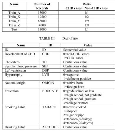
TABLE II. TRAINING AND TESTING DATA SETS
Name Number of
Records
Ratio
CHD cases : Non-CHD cases
Train_A 13000 1:1
Train_X 19500 1:2
Train_Y 65000 1:9
Train_Z 4000 1:9
Test 13000 1:1
TABLE III. DATA ITEM
Name ID Value
ID ID Sequential value
Development of CHD CHD 0=non-CHD cases
1=CHD cases
Cholesterol TC Continuous value
Systolic blood pressure SBP Continuous value
Left ventricular DBP Continuous value
Hypertrophy LVH 0=negative
1=define or positive
National origin ORIGIN 0=native-born
1=foreign-born
Education EDUCATE 0=grade school or less
1=high school, not graduate 2=high school, graduate 3=college or more
Smoking habit TABACO 0=never smoked
1=stopped 2=cigar or pipe 3=tobacco(<20/day); 4=tobacco(20/day=<)
Drinking habit ALCOHOL Continuous value
The CHD_DB consists of four training data sets and one testing data set as shown in Table II. The number of records
and the ratio of CHD cases to non-CHD cases are different between the four training datasets. Each record contains 1 sequential value, 5 desecrate values and 4 continuous values, 10 items in total. ID is index information of patient and not used for training or testing. Development of CHD (CHD) is the class information that shows the patient is CHD cases or non-CHD cases. Other 8 items are real value of test for coronary heart disease. The prognosis of coronary heart disease is the problem of 2 class classification whether the record is CHD cases or non-CHD cases from 8 test values.
Each test item of CHD_DB has different average and variance. We normalized each value so that each item has same average and variance equals 1.0. The normalized value xi of ith
item is defined from the real value Xi as follow:
min
X
X
x
i i i i−
−
=
σ
(23)where X is arithmetic mean of ith item, σ is standard deviation i
of ith item and min is minimum normalized value in each item and each record.
B. Applying Clustering Algorithm for Classification
When applying the clustering algorithm for supervised classification, the clustering result is not matched to the teaching classes. Therefore the clusters are necessary to be labeled from the teaching class labels.
In this paper we define the class labels by the frequency based probability. Let the input data set be S = {xi}, i = 1,…, N;
where xi is real vector, the number of cluster be K, the set of
cluster be a = {ak | ak ∊ S, ak ≠ φ, ∪a = S, ak ∩ ak’) = φ,}, k, k’
= 1,…, K, k ≠ k’; and the number of class be C, the set of class label be Y = {y},y = 1,…, C. The teaching class labels Y obtains function (24) and the clustering result obtain function (25).
( )
if
y
=
x
(24)( )
if
k
=
'
x
(25)The labeling of the cluster is show as following equation.
( )
k
g
y =
(26)We define g(k) from frequency based probability P(y|k). The probability P(y|k) is derived from function (24) and (25):
(
y
k
)
P
k
g
y|
max
arg
)
(
=
(27)(
)
k ka
Y
k
y
P
|
=
(28)where Yk is the set of class labels Yk={ f(xi) | xi ∊ ak }.
C. Applying Adaptive Tree Structured Clustering method for Prognosys of Coronary Heart Disiease
In this paper we applied proposed adaptive tree structured clustering method to 4 different training data sets show in table II and calculate the classification accuracy for the test data set.
In this experiment, we used following parameters for proposed clustering method if there is no annotations. For
θ(0)=0.04, θ’=0.75,φ(0)=0.01, φ’=0.75, ς=0.0 was used. For
the steps of SOM training the following SOM was used. A 9x6 competitive layer was initialized using random values. For the determining of the winner unit we use Euclidian distance. For the neighborhood function hcj we use the Gaussian type. The
following parameters were used, ∆t=10, τ=100, λ(0)=0.1,
λ’=0.9995, σ(0)=9, σ’=0.999 and H=1 was used.
In the first experiment, we evaluated the effectiveness of 3 parameters of proposed clustering method. In this experiment, Train_A was used for training data set. Train_A and Test was used for testing data set.
Figure 1 shows the change of classification accuracy with increasing map size M that the number of SOM competitive layer’s units. The vertical axis is the classification accuracy and the horizontal axis is map size. This result shows that the dependence of map size for the classification accuracy is very low. In this experiment, the better classification accuracy was occurred when smaller map size because the map size has complex relation to the other parameters and the other parameter was optimized for small map size.
Figure 2 and 3 show the results of the classification accuracy and the calculation time with increasing the initial value of SOM training termination thresholds φ(0). The increasing termination thresholds φ causes that each node SOM terminate the training in less training time steps. In the result of the change of classification accuracy shown in figure 2, the dependence of SOM training step for the classification accuracy is very low. Moreover, in the result of figure 3, the calculation time was decreased with increasing the thresholds
φ(0). The decreasing of calculation time is less in low
thresholds φ(0). This is due to increase the frequency of re-clustering step.
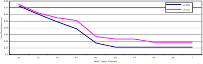
Figure 4 shows the change of classification accuracy with increasing the initial value of node creation threshold θ(0). The increasing the node creation threshold θ causes decreasing obtained number of cluster. Consequently, the classification accuracy is increasing shown in figure 4. In the point of decreasing the change in classification accuracy, we can find the optimal node creation threshold θ(0). In this case, The optimal node creation threshold θ(0) is 0.4.
In the 1st experiment, we confirmed that there was a large difference in the results between separate runs. It is explained that the difference of result is occurred from the dependence of the input data subset of each node. The training steps of each node SOM is less than input data subset in the node near the root. The re-clustering step was applying to improve the deference of result by the verifying data set. However we are necessary to investigate the method for verifying the tree structure in the future.
0.6 0.61 0.62 0.63 0.64 0.65 0.66 0.67 25 36 49 64 81 100 121 144 169 196 Map Size C la ss ifi c at io n A c c ur ac y Train Data Test Data
Figure 1. Change of Classification Accuracy and Map Size
0.6 0.61 0.62 0.63 0.64 0.65 0.66 0.01 0.01 0.02 0.02 0.03 0.03 0.04 0.04 0.05 0.05
End Training Threshold
C la ss ifi c at io n A cc u ra c y Train Test
Figure 2. Change of Classification Accuracy and End Training Threshold
0 100 200 300 400 500 600 0.01 0.01 0.02 0.02 0.03 0.03 0.04 0.04 0.05 0.05 End Training Threshold
T im e (s e c )
Figure 3. Change of Calculation Time and End Training Threshold
0.6 0.61 0.62 0.63 0.64 0.65 0.66 0.67 0.68 0.1 0.2 0.3 0.1 0.5 0.6 0.7 0.8 0.9 1
Node Creation Threshold
C la ss ifi c at io n A c c ur ac y Train Data Test Data
Figure 4. Change of Classification Accuracy and Cluster Size TABLE IV. COMPARISON OF TRAINING DATA SET
Classification Accuracy
Name of Training Data Set Training Data Set Testing Data Set
Train_A 0.67 0.66
Train_X 0.69 0.59
Train_Y 0.9 0.65
Train_Z 0.9 0.63
In the next experiment, we compare the 4 different data sets shown in Table II. The number of records and the class ratio are different in each training dataset. Table IV shows the comparison result by the difference of training data set. This result is the best result of 10 separate runs.
In the result of training data set, Train_Y and Train_Z gave very high classification accuracy. This is due to the class ratio of training data set. In the result of testing data set, Train_A gave the best result. This result shows the dependence of class ratio is high for the proposed clustering method. When there is difference of class ratio, we confirmed that it is necessary to
increase the number of nodes in order to improve the classification accuracy.
V. CONCLUSION
In this paper, we applied adaptive tree structure clustering method for prognosis of coronary heart disease. Through the computer simulation, we showed the characteristics of the proposed clustering method for applying to real complex data. When applying the basic SOM with large map size (about 100x100) or the agglomerative hierarchical clustering methods with Lance Williams update function, the training data sets is not computable within a feasible time. When using the SOM with 30x20 map size, the classification accuracy is 0.62. Compared with these result of other clustering methods, the proposed clustering method could obtain better results with faster computation.
In the result of classification accuracy show in Table IV, about 20 clusters and similar tree structures were obtained in the separate runs. For future works, we plan to investigate the knowledge acquisition method from the extracted tree structure using correlation between cluster of each branch and each element of input vector, in order to find the decision criteria at each branch.
In this experiment, we confirmed that there was a large difference in the results between separate runs. This problem is thought to occur from the dependence of the input data of each node and causes decreasing classification accuracy. In the future, for improve this problem, we investigate 2 different approaches: introducing a method for verifying the tree structure, and applying an ensemble learning method. We expect that verifying the tree structure is an important procedure because the dependence of proposed clustering result is very strong in the nodes near the root. For verifying tree structure, we investigate the method of supervised clustering or semi-supervised clustering. We plan to apply the ensemble learning method to SOM learning and clustering in each node. Additionally we investigate the implementation of ensemble clustering method with distributed computing.
REFERENCES
[1] T. Kohonen,Self-organizing maps, Berlin, Springer, 1995
[2] Pasi Koikkalainen, Progress with the tree-structured self-organizing map, 11th European Conf. on Artificial Intelligence, pages 211-215, 1994 [3] Ross Quinlan, C4.5: Programs for Machine Learning, Morgan
Kaufmann Publishers, 1993
[4] Takashi Yamaguchi, Takumi Ichimura, Kenneth J. Mackin, Adaptive Tree Structured Clustering Method using Self-Organizing Map, Joint 4th International Conference on Soft Computing and Intelligent Systems and 9th International Symposium on advanced Intelligent Systems, 2008 [5] Machi Suka, Takumi Ichimura, Katsumi Yoshida, Development of
Coronary Heart Disease Databases, Proc. of the 8th International Conference on Knowledge-Based Intelligent Information & Engineering Systems (KES2004), Vol.2, pp.1081-1088, 2004
[6] J. MacQueen, Some methods for classification and analysis of multivariate observations, Proc. of the fifth Berkeley symposium on mathematical statistics and probability. vol.I Statistics, p.281-297, 1967 [7] G.N.Lance and W.T.Williams, A general theory of classificatory sorting