Abstract
The upper and lower limits of the reference range of the QT interval (QT) of the electrocardiogram (ECG) were determined using 2529 healthy young males. The QT were classified into 10 classes by the value of the paired RR interval (RR) observed in the same ECG. In each class, the 2.5th and 97.5th percentiles of the conditional distribution of QT were determined as point and interval estimates by the bootstrap method. Using these estimates, the upper and lower limits of the reference range of QT in all RR ranges from 0.6 to 1.5 s were approximated as QTupper limit=436×RR0.35 and QTlower limit=375×RR0.28, respectively. In each class, the 95% confidence intervals (CI) of the upper and lower limits were also estimated. Low reliability was shown by the wide CI of the limits in both extremes of RR range when a sufficient sample size cannot be obtained.
Key words: bootstrap, QT interval, reference range, outliers, tails of distribution, interval estimation
1. Introduction
Reference values (footnote 1) for ECG parameters are usually presented as a set of point estimates of the mean, upper and lower limits. However, since the variance of these values are likely to change depending on the sample size used in the estimation, it is difficult to know the reliabilities of the limits only from the point estimates.
In our previous studies〔1〕〔2〕, we had considered that the reliabilities of the limits could be
quantitatively described based on the length of the 95% confidence intervals (CI) of the limits, and had presented these limits not only as point estimates, but also as interval estimates. Since we could not prepare enough samples for non-parametric study, we assumed the normality of the conditional distribution of QT and approximated the 97.5th and 2.5th percentiles of the
Interval estimation of the upper and lower limits
of the reference range of the QT interval
in resting electrocardiograms by the bootstrap method
Hideo MIYAHARA Hiroshi GOTO
1 We use the terms ‘reference range’ and ‘outlier’ in place of ‘normal’ and ʻabnormal’, respectively, in describing the QT. The reference range of the QT was established from the 2.5th (lower limit) and 97.5th percentiles (upper limit) of measurements in healthy subjects. Measurements that exceeded the upper limit or fell below the lower limit of this range are referred to as outliers.
distribution as the mean ±1.96 sigma of the distribution. Following these studies, we〔3〕 added
new cases from the same institution as that in the previous studies and we had estimated the upper and lower limits with CIs, without assuming the normality of the conditional distribution of QT. In the present study, we summarized the series of our previous reports and presented the exponential equation approximating the upper and lower limits of the QT interval (footnote 2) to be useful for clinical trials. We, also showed how to set the reference value with confidence interval for clinical tests by the bootstrap method.
2. Subjects and Methods
A 12-lead electrocardiogram (ECG) was recorded for 2609 healthy Japanese men aged 20 to 35 years old as a part of screening for candidacy in a phase 1 clinical trial. The screening was performed from March 2006 to March 2009. The RR for each case was determined by averaging the RRs of all leads measured from normal and noise-free beats of the 10-s ECG recording. QT was measured using QT analysis software (FCP-7431 Version S) provided by Fukuda Denshi. After excluding 80 cases who did not meet the enrollment criteria (see Appendix), 2529 cases were used for the study. The mean and standard deviation of the age of the 2529 subjects were 24.3 and 3.8 years old, respectively.
The joint distribution of RR and QT was used to determine a linear regression equation for
QT in terms of RR:
QTL=α×RR+β (2.1)
and an exponential regression equation for QT:
QTE=γ×RRδ. (2.2)
The coefficients, α and γ, intercept β, and exponent δ of these equations were determined using the least squares method.
The RR range (0.600 to 1.500 s) corresponding to the enrollment criteria for the clinical trial was divided into 10 classes. To compensate for the fewer samples at both ends of the RR, the class lengths at both ends were broadened. Thus, the lower and upper limits of the lowest RR class were set at 0.600 and 0.7375 s, respectively, and the limits of the highest RR class were set at 1.3375 and 1.500 s, respectively. The limits of the other 8 intervals were graduated in 0.075-s intervals from the upper limit of the lowest interval. RR=1 s occurred in the interval between 0.9625 and 1.0375 s. The lower and upper limits of the 10 intervals are shown in Table 1. Each subject was classified into one of the 10 classes based on their RR. The value of RR for each case
2 The QT interval represents electrical depolarization and repolarization of the left and right ventricles. On the ECG recording, the QT interval (QT) is defined as the time interval from the onset of one QRS complex to the end of the T wave of the same QRS complex. Since the QT interval is dependent on the heart rate (the faster the heart rate the shorter the QT interval), the reference value of QT was given as a function of RR, explained below. The RR interval (RR) is defined as the time interval from the onset of one QRS complex to the onset of the next QRS complex.
in the same class was replaced with the class value of the interval, whereas the actual values of
QT were used in the analysis. Using the bootstrap method〔4〕, the median, lower limit and upper
limit of the reference range of QT in each class were estimated as follows:
Step 1: The samples corresponding to the sample size in the i-th class (ni ; i=1, 10) were
repeatedly sampled from the same class and a set of QT populations consisting of ni cases was
constructed. The same procedure was repeated j times for the same subjects in the i-th class to produce j sets of QT populations consisting of ni cases (BSik : k=1,..,j). The number of bootstrap
samples (j) was set at 1000 in this study.
Step 2: The 2.5th percentile (Lik ; k=1,..,j) was determined in each of the j sets of BSik for
each i.
Step 3: The 2.5th (L2.5i), 50th (L50i), and 97.5th (L97.5i) percentiles of j samples of Lik were
determined in each class. L50i was defined as the estimated lower limit of the reference range of QT in the i-th class. L2.5i and L97.5i were defined as the lower and upper limits of the CI of L50i, respectively.
Step 4: Similarly to step 2, the 50th (Mik ; i=1,..,10, k=1,..,j) and 97.5th (Uik; i=1,..,10, k=1,..,j) percentiles were determined in each of the j sets of BSik.
Step 5: Similarly to step 3, the 2.5th (M2.5i), 50th (M50i), and 97.5th (M97.5i) percentiles of
j samples of Mik were determined in each class. M50i was defined as the median reference value
of QT in the i-th class, and M2.5i and M97.5i were defined as the lower and upper limits of the
CI of M50i, respectively. Similarly, the 2.5th (U2.5i), 50th (U50i), and 97.5th (U97.5i) percentiles
of j samples of Uik were determined in each class. U50i was defined as the upper limit of the
reference value of QT in the i-th class, and U2.5i and U97.5i were defined as the lower and upper
limits of the CI of U50i, respectively.
Step 6: Using 10 pairs of the class value from the i-th class of the RR and U50i (i=1,..,10),
an exponential regression equation for the upper limit of the reference range of QT was estimated in terms of RR as follows:
QTupper limit=c×RRd (2.3)
The coefficient c and exponent d of the equation were determined using the weighted least squares method.
Step 7: Similarly to step 6, exponential regression equation for the median;
QTmedian=e×RRf (2.4)
and lower limit of the reference range of QT;
QTlower limit=g×RRh (2.5)
were estimated in terms of RR.
We compared the detection rate at both extremes with the anticipated rate of 2.5% after identifying outliers in the subject population using the criteria.
gave written informed consent before starting the study. IBM SPSS Statistics (ver. 19) and Microsoft Excel 2003 SP2 were used for statistical analysis.
3. Results
3.1 Joint distribution of RR and QT
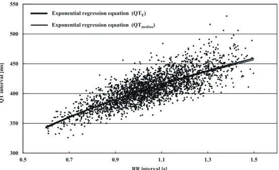
The RR and QT intervals ranged from 0.60 to 1.50 s and from 326 to 530 ms, respectively. Hereafter, the units of QT and RR are ms and s, respectively. The joint distribution of RR and
QT in the 2529 cases is shown in Figure 1. The mean of the conditional distribution of QT for a
given RR increased curvilinearly with the increase of RR. The correlation coefficient between
RR and QT was 0.78. A linear regression equation for QT in terms of RR corresponding to Eq.
(2.1);
QTL=126.5×RR + 276.0 (3.1)
was obtained with a root mean square error (RMSE) of 16.36 ms over all subjects. Similarly, an exponential regression equation for QT in terms of RR corresponding to Eq. (2.2);
QTE=403.3×RR0.32 (3.2)
was obtained with an RMSE of 16.32 ms.
The median of the QT distribution (= M50i) was compared with the arithmetic mean
(Mean) for each of the 10 classes (Table 1). M50i was less than Mean in each class, which suggests
that the conditional distribution of QT slightly leaned toward the shorter end. In 9 of 10 classes excepting class 5, the length of the upper half of the range of the QT (U50i-M50i) was slightly
longer than that of the lower half of the range (M50i-L50i). In class 5, the length of the upper
half was equal to that of the lower one.
However, the difference between M50 and Mean in each class was minimal and the values agreed to two significant figures. The ranges of the CI of the median (M97.5i-M2.5i) were
from 3 to 10 ms and did not increase with RR, but with the inverse of the sample size. QTmedian
was estimated as
QTmedian=403.03×RR0.31 (3.3)
The coefficient of 403.03 and exponent of 0.31 were very close to the respective values for QTE .
3.2 Point and interval estimation of the upper and lower limits of the QT reference value
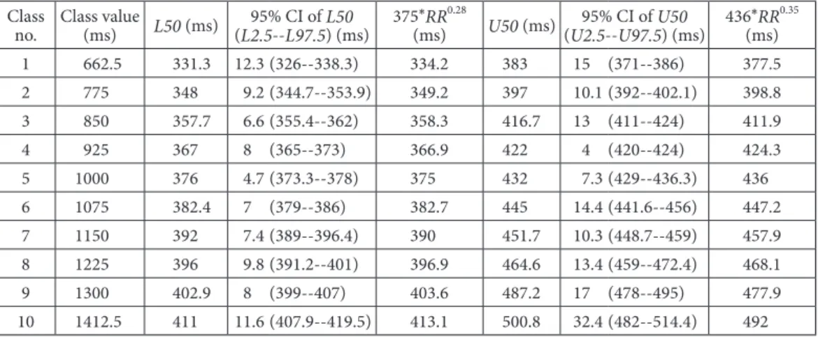
The upper limit of the reference value of QT in the i-th class (U50i) and the upper (U97.5i)
and lower (U2.5i) limits of the CI of U50i (i=1,..,10) estimated for each of the 10 classes using
the bootstrap method are shown in Table 2. In the 5th class (class value 1 s, sample size 491),
U2.5i, U50i, and U97.5i were 429.0, 432.0 and 436.3 ms, respectively, and the length of the CI
was 7.28 ms. Similarly to M50i , U50i increased along with RR. The lengths of the CIs broadened
In Step 6 above, the equation;
QTupper limit=436×RR0.35 (3.4)
was obtained for the upper limit of the reference range of the QT population. The RMSE of this equation was 5.98 ms. The upper and lower limits of the CI of QTupper limit in the i-th class were
approximated using U97.5i and U2.5i, respectively. The value of QTupper limit exceeded U97.5i=4 by
0.2 ms in the 4th class, but remained within the CIs of U50i in all other classes.
Using the same procedure for the upper limit, L50i and the upper (L97.5i) and lower (L2.5i)
limits of the CI of L50i (i=1,..,10) were estimated for each of the 10 classes (Table 2). Similarly
to M50i and U50i, L50i increased along with RR. In the 5th class, L2.5i=5, L50i=5 and L97.5i=5
were 373.3, 376 and 378 ms, respectively, and the length of the CI was 4.75 ms. The lengths of the CIs broadened to 12 ms in the shorter and longer RR classes, but showed no increasing or decreasing trend with respect to RR. Using similar steps to estimate QTupper limit, the exponential
equation;
QTlower limit=375×RR0.28 (3.5)
was obtained for the lower limit of the reference range of the QT population. The RMSE of this equation was 1.63 ms. The upper and lower limits of the CI of QTlower limit in the i-th class were
approximated using L97.5i and L2.5i, respectively. The value of QTlower limit remained within the
CIs of L50i in all 10 classes. Curves representing Eq. (3.4) and Eq. (3.5) and the CIs of the upper
and lower limits of the reference range are shown with the plot of the joint distribution of RR and QT in Figure 2.
The length of the CI of the upper limit (U97.5i-U2.5i) was longer than that of the lower
limit (L97.5i-L2.5i) in 9 of 10 classes excepting class 4. In class 4, the length of CI of U50i=4
was exceptionally short (4ms) and shorter than that of L50i=4(Table 2).
3.3 Detection of outliers in the target population
Using Eq. (3.4), 62 of the 2529 cases (2.45%) with QT exceeding the limit were identified as
outliers with longer QT. Similarly, using Eq. (3.5), 61 cases (2.41%) fell below the limit and were identified as outliers with shorter QT. The other 2406 cases were located between the two limits and thus had QT within the reference range.
4. Discussion
Since the definition of the reference value was generally established by the range between the 2.5th and 97.5th percentiles of measurements, it was preferable to determine both limits directly from the sufficient numbers of samples.
Pavlov et al〔5〕 compared the parametric and nonparametric approaches for determining the
nonparametric approach. Linnet〔6〕 also suggested that nonparametric reference interval
estimation at small to moderate sample sizes (<120) was associated with a large degree of uncertainty.
We had shown that the marginal distribution of RR of the healthy population could be
approximated by a normal distribution〔1〕. So, we expected that the sample size at both the
shorter and longer ends of RR would be much less than those in the intermediate classes. In the previous study using 1276 cases〔2〕, the number of cases for the RR range less than 0.737 s was
30, whereas that for the RR range longer than 1.337 s was 57. To avoid the deterioration of the reliability, we assumed the normality of the conditional distribution of QT, and approximated the 97th and 2.5th percentiles of the distribution as the mean ±1.96 sigma of the distribution.
In the present study, we doubled the number of cases which were from the same institution as that in the previous studies〔2〕〔7〕〔8〕. As a result, the number of cases for the RR range less than
0.737 s increased from 30 to 66, whereas that for the RR range longer than 1.337 s increased from 57 to 107. To keep the sufficient sample size, we had expanded the class width in both ends of the RR range twice as compared with our previous studies. However, the sample size was still not enough to fulfill the Linnet’s requirement〔6〕.
In clinical medicine, many laboratory data had been approximated by normal or log-normal distribution to estimate their reference ranges.
Since p-value of Shapiro-Wilk test was 0.27, we had assumed normality of the data in class 5, and estimated mean 404.13 and standard deviation 15.22 ms. The upper and lower limits of the reference range defined as the mean ±1.96 sigma were thus 433.96 and 374.30 ms. Provided normal assumptions hold, we also calculated CI for these limits. The CIs of upper and lower limits were from 431.63 to 436.29 and 371.97 to 376.63 ms.
As an alternative approach, assuming the normality of the log-transformed data in the same class 5 (p-value of Shapiro-Wilk test was 0.46), we had estimated mean 2.01 and standard deviation 0.016. The lower limit in the transformed data was 2.57, corresponding to a QT of 375.12 ms, and the upper limit was 2.64, corresponding to 434.76 ms. The CIs in linear scale were 432.22 to 437.22 ms for the upper limit and 372.99 to 377.31 ms for the lower limit.
However, since there was no reason to suppose that all variables followed a normal distribution, we estimated the limits of the reference range non-parametrically.
Using the bootstrap method, we directly estimated the upper and lower limits. They were 432 and 376. Both limits estimated non-parametrically well agreed with those estimated parametrically.
The CIs of upper and lower limits estimated by the non-parametric approach were 429.00 to 436.28 and 373.25 to 378.00 ms, respectively. The length of CI of upper limit was 2.53 ms longer than that of lower limit.
if we assumed the normality of the data. On the other hand, it is known that the length of CI of upper limit is longer than that of lower limit under the assumption of the log-normality of the data. In fact, we found that the length of CI of the upper limit was 0.69 ms longer CI than that of the lower limit. However, the difference was much shorter than we obtained using non-parametric approach.
From these results, we found that we could estimate the limits of reference range using the parametric approach if the data were well approximated by the assumed distribution. However, we also found that the assumed distribution could not be applied to data around the limits even if the distribution well fitted to the samples in the central region. Samples in the tails might have a unique characteristics from those in the central region, and we had to estimate the variance of the limits independently.
The bootstrap method can be easily applied to such a purpose without assuming any type of the distribution. We could estimate the length of the CI of the limits of reference range and find the difference of the length of the CI between upper and lower limit. Using these CIs, we could rate the reliability of the limits.
It is needed further studies to elucidate the reasons why the CI of the upper limit tended to lengthen than lower one.
Summary
The current investigation of the relationship between the RR and QT intervals in resting ECGs of 2529 healthy young Japanese men showed that the upper and lower limits of the reference range of QT in the RR ranges from 0.8 s to 1.3 s were well approximated by the pair of exponential equations QTupper limit=436×RR0.35 and QTlower limit=375×RR0.28, respectively. In this
study, we did not assume the normality of the conditional distribution of QT in each class, and estimated the upper and lower limits of the reference range of QT as 97.5th and 2.5th percentiles, respectively. We also estimated confidence intervals of these border points non-parametrically. These intervals could be used for evaluating the reliability of the limits of the reference range. Using non-parametric approach, we found that the dispersion of the upper limit of QT was larger than that of the lower limit.
Acknowledgements
We acknowledge the many contributions to preparation of data made by the staff of the Tsukuba International Clinical Pharmacology Clinic.
References
rest electrocardiograms of healthy young Japanese men. Japanese Journal of Electrocardiology, 27, 596–607, 2007, (in Japanese)
〔2〕Miyahara, H., Goto, H., Shimizu, K., & Ikeda, N.: Application of the bootstrap method in the determination of the reference value of clinical laboratory data. The Japanese Journal of Behaviormetrics, 40 (2), 89–95, 2013 (in Japanese).
〔3〕Miyahara, H Goto, H., Hemmi, O, Ikeda, N.: The upper and lower limits of the reference range of the QT interval in rest electrocardiograms of healthy young Japanese men. Bulletin of Toyohashi Sozo University 16, 105–114, 2012.
〔4〕Efron, B., & Tibshirani, R.J.: An introduction to the bootstrap. Chapman & Hall/CRC, 1998. 〔5〕Pavlov, I.Y., Wilson, A.R., & Delgado, J.C.: Reference interval computation: which method (not) to
choose? Clinica Chimica Acta, 413, 1107–1114, 2012.
〔6〕Linnet, K.: Nonparametric estimation of reference intervals by simple and bootstrap– based procedures. Clinical Chemistry, 46, 867–869, 2000.
〔7〕Goto, H., Mamorita, N., Ikeda, N., Miyahara, H.: Estimation of the upper limit of the reference value of the QT interval in rest electrocardiograms in healthy young Japanese men using the bootstrap method. Journal of Electrocardiology. 41 (6), 703e1–703e10, 2008.
〔8〕Miyahara, H., Goto, H., Ikeda, N.: Estimation of the upper limit of the QT interval reference value by the bootstrap method. Bulletin of Toyohashi Sozo University 15, 87–97, 2011 (in Japanese).
Appendix
Exclusion criteria of the institution and number of cases excluded from the study.
ECG findings Exclusion criteria of institution Number of cases
Sinus tachycardia >100 beats/m 5
Sinus bradycardia <40 beats/m 2
Left axis deviation <30 degree 13
Right axis deviation >110 degree 12
Myocardial ischemia 2
Complete right bundle blanch block Pattern + QRS duration>135 ms 5
Intraventricular conduction disturbance QRS duration>135 ms 7
Short PR interval PR interval<80 ms 1
First degree atrioventricular block PR interval>260 ms 4
Atrioventricular junctional rhythm 15
Premature ventricular contraction 5
Premature supraventricular contraction 3
Escaped beat 3
Second degree atrioventricular block 1
Third degree atrioventricular block 1
WPW 1
300 350 400 450 500 550 0.5 0.7 0.9 1.1 1.3 1.5 Q T in te rv al [m s] RR interval [s] Exponential regression equation (QTE) Exponential regression equation (QTmedian)
Figure 1. Relationship between QT and RR intervals in resting ECGs of 2529 healthy young Japanese men. Curves representing the exponential regression equations for QT (QTE) and the median of QT (QTmedian) are shown as bold and thin lines,
respectively.
Figure 2. CIs of the upper and lower limits of the reference range. U50i (×) and L50i (●)
obtained in each RR class using the bootstrap method are shown with an intermediate line. Curves representing the exponential regression equations for
QTupper limit, QTmedian and QTlower limit are shown as a thick, intermediate and thin
Table 1. Class value, range, sample size, arithmetic mean, SE of mean, median, and range of CI of median, and QTmedian corresponding to each RR class.
RR interval QT interval
Class
no. No. of cases Class value (ms) Range (s) Mean (ms) SE of mean (ms) Median (ms)
Range of 95% CI of Median (ms) QTmedian (ms) 1 66 662.5 0.5995--0.7375 356.05 1.64 356 8.5 354.68 2 120 775 0.7375--0.8125 373.08 1.17 372 5.5 372.31 3 215 850 0.8125--0.8875 384.07 1.04 382 3.0 383.10 4 321 925 0.8875--0.9625 394.05 0.81 393 4 393.26 5 491 1000 0.9625--1.0375 404.13 0.69 404 3 402.85 6 458 1075 1.0375--1.1125 412.36 0.78 411 3 411.97 7 335 1150 1.1125--1.1875 421.50 0.88 420 5 420.65 8 257 1225 1.1875--1.2625 428.47 1.14 426 5 428.95 9 159 1300 1.2625--1.3375 440.63 1.74 439 6 436.91 10 107 1412.5 1.3375--1.4665 450.38 2.21 450 10 448.27
Table 2. Upper and lower limits of the reference value of QT in each class estimated using the bootstrap method. The values of QTupper limit and QTlower limit for the class value of each RR
were also included.
Class
no. Class value (ms) L50 (ms) (L2.595% CI of --L97.5L50) (ms) 375*RR
0.28
(ms) U50 (ms)(U2.595% CI of --U97.5U50) (ms) 436*RR
0.35 (ms) 1 662.5 331.3 12.3 (326--338.3) 334.2 383 15 (371--386) 377.5 2 775 348 9.2 (344.7--353.9) 349.2 397 10.1 (392--402.1) 398.8 3 850 357.7 6.6 (355.4--362) 358.3 416.7 13 (411--424) 411.9 4 925 367 8 (365--373) 366.9 422 4 (420--424) 424.3 5 1000 376 4.7 (373.3--378) 375 432 7.3 (429--436.3) 436 6 1075 382.4 7 (379--386) 382.7 445 14.4 (441.6--456) 447.2 7 1150 392 7.4 (389--396.4) 390 451.7 10.3 (448.7--459) 457.9 8 1225 396 9.8 (391.2--401) 396.9 464.6 13.4 (459--472.4) 468.1 9 1300 402.9 8 (399--407) 403.6 487.2 17 (478--495) 477.9 10 1412.5 411 11.6 (407.9--419.5) 413.1 500.8 32.4 (482--514.4) 492