GENERATORS AND RELATIONS FOR THE MAPPING CLASS GROUP OF THE HANDLEBODY OF GENUS 2(Analysis of Discrete Groups II)

(1)

GENERATORS AND RELATIONS FOR THE MAPPING

CLASS GROUP OF THE

HANDLEBODY

OF GENUS 2

SUSUMU HIROSE Department of Mathematics Fuculty of Science and Engineering

Saga University

INTRODUCTION

A handlebody ofgenus$g,$ $H_{g}$, is anorientable 3-manifold, which is constructed ffoma

3-ball with attaching$g1$-handles. Let $D_{\dot{i}}ff^{+}(H)g$ be thegroup oforientationpreserving diffeomorphisms on $H_{g},$ $\mathcal{H}_{g}$ be a groupwhich consists of isotopy classesof

$D_{\dot{i}}ff^{+}(H)g$

.

The groups $\mathcal{H}_{g}$

are

interesting objects because of their relationships with Heegaard

splittings of3-manifolds and outer automorphism group offree groups. In this paper, we give a presentation of$\mathcal{H}_{2}$

.

Before we state this presentation, we set notations used

there. We indicate an element of$Diff^{+}(H_{g})$ by figure like left hand side of Figure 1,

in this figure, the left hand side figure denotes an element given in the right hand side figure.

The $\mathrm{s}\mathrm{y}\mathrm{m}\mathrm{b}_{\mathrm{o}1}\Leftrightarrow \mathrm{m}\mathrm{e}\mathrm{a}\mathrm{n}\mathrm{s}$ commute with. If _$L,$$M,$$N$ are any

elements of$\mathcal{H}_{g}$, a relation

$L\Leftrightarrow M,$ $N$ means that $LM=ML,$ $LN=NL$

.

In _this paper,

we

_{consider that the}

group $\mathcal{H}_{g}$ acting on $H_{g}$ from the right.

Theorem 1. Leta, $b,$ $c,$ $d,$ $t,$ $e,$ $f$ be the elements

of

$\pi_{0}(Diff^{+}(H_{2}))$ by the elements

of

$D_{\dot{i}}ff^{+}(H2)$ indicated in Figure 2. The group _{$\pi_{0}(Diff^{+}(H_{2}))$} admits a _presentation with generators a, $b,$ $c,$ $d,$ $t,$ $e,$ $f$ and defining relations,

(2)

–

$\pi-\mathrm{r}\mathrm{o}\mathrm{t}\mathrm{a}\mathrm{t}\mathrm{i}\mathrm{o}\mathrm{R}$ along the

indicated axis FIGURE 1 $\alpha$ $\mathrm{b}$ $\mathrm{c}$ $\tau$ $\mathrm{e}$ FIGURE 2

(3)

$e^{2}=f^{2}=1$, $fbfb^{-1}fb=ca^{-1}de,$$aba^{-}1b^{-}1=d^{22}c$, $dad^{-1}=d^{2_{C}2}a^{-},$$d1b-1d-1=d^{2}cb2$, $t-1bt=ba,$ $ftf=C-1,$$e=fd-1fd$, $c\Leftrightarrow a,$$b,$$d$, $e\Leftrightarrow a,$_{$b,$ $c,$}$d,t,$$f$, $t\Leftrightarrow a,$$c,$$d$, $f\Leftrightarrow a^{-1}t,$ $d^{2}$

.

Contents are asfollows: insection 1, weset notations, and reviewmethod, by Brown,

to get a presentation of a group which act simplicially on a simply connected

CW-complex, and introduce a simply connected $\mathrm{C}\mathrm{W}$-complex where $\mathcal{H}_{2}$ acts. In section 2,

we obtain a presentation of subgroups of $H_{2}$ which is used to prove Theorem 1. In

section 3,

we

prove Theorem 1. In section 4,

we

check this presentation by showing

that there is

a

surjection from $\mathcal{H}_{2}$ to $SL(2, \mathbb{Z})$ and injectionwhich is the inverse of this

surjection.

1. PRELIMINARIES

In this section,

we

set notations and review tools used in this paper.

1. Notations. Let $X$ be any oriented manifold, and $K_{1},$

$\ldots$ ,$K_{n},$$K_{n+1}$ be subsets of

X. We introduce

a

notation

as

follows,

$Diff^{+}(X, K_{1}, \ldots, K_{n},rel(K_{n+1}))=$

.

For abbreviation,

we

denote $Diff^{+}(X, K_{1}, \ldots , K_{n}, rel(\emptyset))$ by $Diff^{+}(x, K_{1}, \ldots, K_{n})$,

(4)

by $Diff^{+}(X)$

.

The set $D_{\dot{i}}ff^{+}(X, K_{1}, \ldots, K_{n}, rel(K_{n+}1))$ has a natural group

struc-ture. In this paper, we consider that the group $D_{\dot{i}}ff^{+}(X, K_{1}, \ldots, K_{n}, rel(K_{n+}1))$ acts

on$X$fromtheright, thatis, for elements$\varphi_{1}$ and$\varphi_{2}$of$Diff^{+}(X, K_{1}, \ldots, K_{n}, rel(K_{n+}1))$,

$\varphi_{1}\varphi_{2}$ means that apply $\varphi_{1}$ first, and apply $\varphi_{2}$

.

The group $\pi_{0}(D_{\dot{i}}ff^{+}(X,$$K_{1},$

$\ldots,$$K_{n}$,

$rel(K_{n+1})))$ consistsof the isotopy classesof$D_{\dot{i}}ff^{+}(X, K_{1}, \ldots, K_{n}, rel(Kn+1))$ and its

group law is induced from that of $Diff^{+}(X, K_{1}, \ldots, K_{n}, rel(K_{n}+1))$

.

Especially, we

denote $\pi_{0}(Diff^{+}(H_{g}))$ by $\mathcal{H}_{g}$

.

In this paper, we give apresentation of$\mathcal{H}_{2}$

.

We denote

by $<a_{1},$ $\ldots.’ a_{n}|>\mathrm{a}.\mathrm{f}\mathrm{r}\mathrm{e}\mathrm{e}$ group generated by $a_{1},$ _$\ldots,$$a_{n}$

.

2. Brown’s method [Br]. Let $G$ be a group, and $X$ be a simply connected

CW-complex on which $G$ acts as cellular homeomorphisms. We call this $X$ as simply

con-nected G-CW-complex. In this paper, we regard the action of $G$ as a right action. There is a method introduced by Brown [Br] to get a presentation of $G$ from asimply connected $G- \mathrm{C}\mathrm{w}_{-}\mathrm{C}\mathrm{o}\mathrm{m}_{\mathrm{P}}1\mathrm{e}\mathrm{X}$

.

In this subsection,

we

review this method.

At first, we need to introduce some notations and terminologies. For any

CW-complex $C$, a $0$-cell of $C$ is called a vertex. A 1-cell of $C$ with an orientation is called an edge. Any edge $e$ has an initial vertex $o(e)$ and a final vertex $t(e)$

.

The notation $\overline{e}$ denote the edgecorresponding to the same 1-cell as $e$ and whose orientationis opposite

to $e$

.

$V(C)$ denote the set of vertices of $C,$ $\Sigma(C)$ denote the set of 1-cells of $C$, and

$E(C)$ denote the set of edges of $C$

.

Rom here to the end of this subsection, $X$ denote a $G- \mathrm{C}\mathrm{w}_{-}\mathrm{C}\mathrm{o}\mathrm{m}_{\mathrm{P}}1\mathrm{e}\mathrm{X}$

.

A 1-cell $\sigma$

of $X$ is called inverted ifthere is an element $g$ of $G$ such that $\sigma g=\sigma$ and

reverse

the

orientation of$\sigma$

.

The notation $\tilde{\Sigma}^{-}$

denote thesetofinverted 1-cellsof$X$, and $\tilde{\Sigma}^{+}$

denote the set of non-inverted 1-cells of$X$

.

A simply conected $\mathrm{C}\mathrm{W}$-complex which consists of $0$-cells and 1-cells is called a tree. A subtree $T$ of$X$ is $\mathrm{c}\mathrm{a}\mathrm{l}\mathrm{l},\mathrm{e}\mathrm{d}$ a tree

of

reprsentatives if $V(T)$ is the set ofrepresentatives of$V(X)/G$, _{and each} _{element of}$\Sigma(T)$ is an element

of $\tilde{\Sigma}^{+}$

.

A tree ofrepresentatives of$X$ is a ‘fundamental domain’ of the action of$G$ on

X. We can give an orientation for each element of $\tilde{\Sigma}^{+}$

(5)

the action of $G$

.

A subset $P$ of _$E(X)$ given in the above manner, is called $\mathit{0}\dot{n}entat\dot{i}on$

of $X$. Let $E^{+}$ be the set of representations of _$P/G$ such that for each

$e\in E^{+}o(e)$ is

an

element of$E^{+}$ and for each 1-cell of_$T$given proper orientation is an

element of$E^{+}$

.

Let $\Sigma^{+}$ be the set of 1-cells of _$X$

which correspond to the elements of $E^{+}$

.

Let $E^{-}$

be the set ofrepresentatives of$\Sigma^{+}/G\sim$ with

an

orientation such that for each

$e\in E^{-}$,

$o(e)\in V(T)$

.

Let $\Sigma^{-}$ be the set of 1-cells of_$X$ which correspond to the

elementsof$E^{-}$

For each $e\in E^{+},$ $t(e)$ may not be an element of $V(T)$, but there is

one

_{and only} one element of$V(T)$ in the orbit of$t(e)$ by the action of $G$

.

We denote this vertexby _$w(e)$

.

Bythe definition of$w(e)$, there is at least one and not unique element $g_{e}$ of$G$such that $w(e)g_{e}=t(e)$. When $e\in E(T)$, we choose $g_{e}=1$. For any $g\in c_{t(e),ggg_{e}}e-1\in G_{w(e)}$

.

Hence, we can define isomorphism $c_{e}$ from $G_{t(e)}$ to $G_{w(e)}$ by $c_{e}(g)=g_{e}gg_{e}^{-1}$

.

Any

element of$G_{e}$ preserve$t(e)$, so we can naturally consider $G_{e}$ as asubgroup of_{$G_{t(e)}$}

.

We

can define in the natural way the injection from $G_{e}$ to _{$G_{w(e)}$}, we denote this injection

also by $c_{e}$

.

For the sake of giving the presentation, we need to present $g_{e}gg_{e}^{-1}$ as an

element of $G_{t(e)}$ for each generator of $G_{e}$.

Each edge $\epsilon$ of $X$, such that $o(\epsilon)\in V(T)$, fall into the following three cases: (1) $\epsilon$

corresponds to a 1-cell in $\tilde{\Sigma}^{+}$

and there is an element $e\in E^{+}$, and an element _{$g\in G$}

such that $eg=\epsilon,$ (2) $\epsilon$ corresponds to a 1-cell in

$\tilde{\Sigma}^{+}$

and there is an element $e\in E^{+}$,

and an element $g\in G$ such that $\overline{e}g=\epsilon,$ (3) $\epsilon$ corresponds to a 1-cell in

$\tilde{\Sigma}^{-}$

In these cases, $\epsilon$ is

as

indicated in the following figures.

(1) $\phi \mathrm{t}\mathrm{J}\overline{\mathrm{e}R\prime-\epsilon}(4)@4*$ $(h\in G_{v}, e\in E+)$

(2) $\Lambda r\mathrm{J}\overline{\mathrm{e}}\mathrm{t}^{\overline{\mathrm{e}}^{1}}\mathit{4}_{\iota^{-}}-\epsilon 0\mathfrak{l}\mathrm{e}\tau_{7^{\overline{\mathrm{e}}}}|*$ $(h\in G_{w}, e\in E+)$

(3) $\wedge’\overline{\mathrm{e}^{\chi\underline{-}}\epsilon}’\iota)\mathrm{x}f_{(}$ ($h\in G_{v},$ $t\in E^{-},$ $t\in G_{\sigma}$ reverse the orientation of $\sigma$)

We can consider $\epsilon$ as a bridge between $T$ and $Tg$ for

some

$g\in G$

.

The above figure indicates the way how to give this $g$ for each $\epsilon$

.

In (1), $g=g_{e}h$, in (2), $g=g_{e}^{-1}h$,

in (3), $g=th.$ Let $\alpha$ be a colsed path in $X$ such that whose base point

(6)

$V(T)$

.

We choose

an

element $g_{\alpha}$ of $G$

as

follows. This path is

a sequence

of edges

$e_{12n}^{\prime_{e\cdots e}}\prime\prime$

.

The first

one

$e_{1}’$ is

an

edge such that $o(e_{1})/=v_{0}\in V(T)$,

we can

obtain

elements $v_{1}\in V(T),$ $g_{1}\in G$ such that $v_{1}g_{1}=t(e_{1})/$ in the above

manner.

The initial

vertex of $e_{2}=e_{2}’g_{1}^{-}1$ is $v_{1}\in V(T)$

.

Hence, in the

same

way, we

can

obtain elements

$v_{2}\in V(T),$ $g_{2}\in G$ such that $v_{2}g_{2}=t(e_{2})$

.

This

means

$t(e_{2}’)=v_{2}g_{2}g_{1}$

.

We continue

this construction successively for other $e_{3}’’,$$e_{4},$ $\ldots$ and $e_{n}’$, then

we can

get a sequence

$g_{1},g_{2},$$\ldots g_{n}$ of elements of $G$ such that $v_{n}gn\ldots g_{2}g_{1}=t(e_{n}’)$

.

In our situation,

$\alpha$ is a

loop,

so

$v_{n}=v_{0}$

.

Hence, $g_{\alpha}=g_{n}\cdots g_{2}g_{1}$ is

a

element of $G_{v_{\mathrm{O}}}$

.

Let

$\hat{G}=()*v\in V^{*}(T)^{c_{v}}$

$(*c_{\sigma})*\sigma\in\Sigma-(*e\in E+<\hat{g}_{\epsilon}>)$

.

In the above construction, $g_{i}$ is aproduct of

$g_{e},$ $t\in G_{\sigma}$ and

$h\in G_{v}$

.

The element $\hat{g}_{i}$ of

$\hat{G}$ is given $\mathrm{h}\mathrm{o}\mathrm{m}g_{i}$ with replacing $g_{e}$ with $\hat{g}_{e}$

.

Let $F$ be the

set ofrepresentatives of 2-cells of X modulo $\mathrm{G}$ such that, for each $\tau\in F,$ $\partial\tau$gothrough

$V(T)$

.

In the above way, we construct $\hat{g}_{\partial\tau}$

.

By the following theorem,

we

can obtain a presentation of$G$

.

Theorem [Br]. In the above situation, $G$ is presented as$\hat{G}$

with the following relations:

(1)

_for

$e\in E(T),\hat{g}_{e}=1$,

(2)

_for

each $e\in E^{+}$ and $g\in G_{e},\hat{g}_{e}i_{e}(g)\hat{g}_{e}^{-}1=c_{e}(g)$, where $i_{e}$

:

_{$G_{e}arrow G_{o(e)}$} is the

indusion and$c_{e}$ : $G_{e}arrow G_{w(e)}$ is the injection given above,

(3)

_for

each $e\in E^{-}$ and$g\in G_{e},$ $i_{e}(g)=j_{e}(g)$, where $i_{e}$ : $G_{e^{\mathrm{e}}}arrow Go(e),$ $j_{e}$

:

$G_{e}\mathrm{c}arrow G_{\sigma}$

are inclusions,

(4)

_for

each $\tau\in F,\hat{g}_{\partial\tau}=g_{\partial\tau}$

.

$\square$

3. The disk complex [Jo]. In this subsection, we introduce simply connected

CW-complex, where the group $\mathcal{H}_{2}$ acts simplicially.

The disk complex $\Delta(H_{2})$ of $H_{2}$ is the simplicial complex whose $m$-simplices are

iso-topy classes of $(m+1)$-tuples $(D_{0}, D_{1}, \ldots, D_{m})$ of essential and pairwise non-isotopic

disjoint disks. In $H_{2}$, there is no

more

than three disks which define

a

simplex. Hence,

$\Delta(H_{2})$ is a 2-dimensional simp\‘iicial complex. By some cut and paste argument,

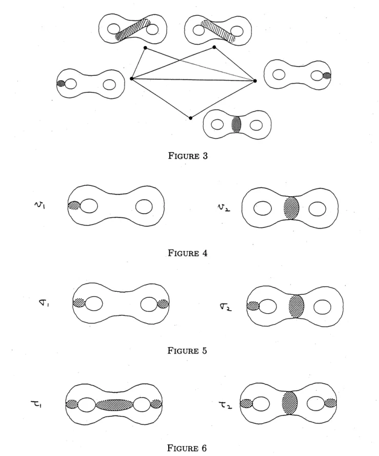
we

(7)

FIGURE 3 $\mathrm{A}f_{1}$ $\mathrm{u}_{\mathrm{L}}$ FIGURE 4 $\nabla_{1}$ $T_{\mathrm{L}}$ FIGURE 5 $\tau_{\mathrm{I}}$ $- \mathrm{c}_{\mathrm{L}}$ FIGURE 6

manifold, because, for each edges, there are more than three faces emanating from this

(8)

$\Theta_{-}$

.

FIGURE 7

FIGURE 8

(1) the set of representatives of $V(H_{2})/\mathcal{H}_{2}$ consists of two elements $v_{1}$ and $v_{2}$ (see

Figure 4),

(2) the set of representatives of 1-cells of$\Delta(H_{2})$ modulo$\mathcal{H}_{2}$ consists of two elements

$\sigma_{1},$ $\sigma_{2}$, one of them $\sigma_{1}$ is inverted and the other $\sigma_{2}$ is non-inverted (see Figure

5),

(3) theset ofrepresentatives of2-cells of$\Delta(H_{2})$ mod $\mathcal{H}_{2}$ consists of 2-elements $\tau_{1},$$\tau_{2}$

(see Figure 6).

Here,

we

make a choice. Let a tree of representatives $T$ be the subcomplex of $\Delta(H_{2})$

which consists of$\sigma_{2},$ $v_{1}$ and $v_{2}$

.

Let $e_{1}$ be anedge which is $\sigma_{1}$ withorientation given in

Figure 7, $e_{2}$ be an edge which is $\sigma_{2}$ with orientation from $v_{1}$ to $v_{2}$

.

We set $E^{+}=\{e_{2}\}$,

$\Sigma^{+}=\{\sigma_{2}\},$ $E^{-}=\{e_{1}\}$ and $\Sigma^{-}=\{\sigma_{1}\}$

.

Since $t(e_{2})\in V(T)$, we choose $g_{e_{1}}=1$ and

$w(e_{2})=t(e_{2})$

.

In the next section, we give presentations for $G_{v_{1}},$ $G_{v_{2}}$ and $G_{\sigma_{1}}$, sets of

generators for $G_{e_{1}}$ and $G_{e_{2}}$

.

2. SUBGROUPS OF $\mathcal{H}_{2}$

In thissection, we will give presentations for the groups which we use to give a pre-sentation for $\mathcal{H}_{2}$

.

Let $D_{1},$ $D_{2},$ $D_{3}$ be disks properly embeddedin $H_{2}$ indicated in Figure

(9)

$\mathrm{c}_{1}$

$c_{L}$

FIGURE 9

8. With these notations, $G_{v_{1}}=\pi_{0}(D\dot{i}ff^{+}(H_{2}, D1)),$ $G_{v}2=\pi_{0}(D\dot{i}ff^{+}(H_{2}, D_{3})),$ $c_{\sigma_{1}}=$

$\pi_{0}(D_{\dot{i}}ff^{+}(H_{2}, D_{1}\cup D2)),$_{$G_{6_{1}}=\pi 0(D\dot{i}ff^{+}(H2, D1, D_{2}))$} and

$G_{e_{2}}=\pi_{0}(Diff^{+}(H_{2,1}D$,

$D_{3}))$

.

Proposition1. Leta,$b,$$c_{1},$ $C_{2},$$d,$$t1,$$t_{2}$ be the elements

of

_{$\pi_{0}(D\dot{i}ff^{+}(H_{2,1}D\cup D2))$} given

in Figure 9 This group admits a presentation with generators a,$b,$$c_{1},$$C_{2},$$d,$$t1,$$t_{2}$, and

defining relations, $t_{1}^{222}=t_{2}=b,$$d=1,$$dt_{1}d=t_{2},$ $dc_{1}d=c_{2}$ $t_{1}^{-1}$at_{$1=t_{2}^{-1}at_{2^{-}}-b-1-a1C_{1}^{-}c22-2$}, $t_{1}\Leftrightarrow t_{2}$, $a\Leftrightarrow c_{1},$$c_{2},$$d$, $b\Leftrightarrow c_{1},$ $c_{2},$$d$, $c_{1}\Leftrightarrow c_{2}$ $t_{1},$ $t_{2}\Leftrightarrow b,$ $c_{1},$$c_{2}$

.

$\square$

(10)

A $\mathrm{b}$ $\mathrm{c}$ $\iota$ $T$ $\mathrm{e}$ FIGURE 10 $=_{-}\iota$ $\mathrm{e}_{\iota}$ $\mathrm{T}_{1}$ X$\iota$ -k; $\mathrm{Y}$ FIGURE 11

10. Thisgroup admits a presentation with generatorsa,$b,$ $c,$$d,$$t,$$e$ anddefining relations,

$aba^{-1}b^{-1}=d^{2}c^{2},$ $dad^{-1}=aba^{-1}b-1da^{-1},bd-1=ab^{-1-1}a$,

$e^{2}=1,$ $t^{-1}bt=ba$,

$e\Leftrightarrow a,$_{$b,$ $c,$ $d,$ $t,$} $t\Leftrightarrow a,$_$c,$$d$,

$c\Leftrightarrow a,$$b,$$d$

.

(11)

Proposition 3. Let $e_{1},$ $e_{2},$ $t_{1},$ $t_{2},$ $r$ be the elements

of

$\pi \mathrm{o}(Diff^{+}(H2, D3))$ given in

Figure 11. This group admits a presentation with generators above 6 elements and defining relations,

$e_{1}^{2}=e_{2}^{-2},$$r^{2}=1,rt_{1}r=t_{2}$,

$re_{1}r=e_{2}^{-1}$, $e_{1}\Leftrightarrow t_{1},e_{2},t_{2}$, $e_{2}\Leftrightarrow t_{1},t_{2}$, $t_{1}\Leftrightarrow t_{2}$

$\square$

Proposition 4. The group $\pi_{0}(Diff^{+}(H2, D1, D_{2}))$ is generated by $e_{1},$ $e_{2},$ $t_{1},$ $t_{2},$ $t_{3}$

given in Figure 11. $\square$

Proposition 5. The group $\pi_{0}(Diff^{+}(H2, D1, D_{3}))$ is generated by$e_{1},$ $e_{2},$ $t_{1},$ $t_{2}$ given

in Figure 11. $\square$

3. A PRESENTATION FOR $\mathcal{H}_{2}$

Let $\hat{G}=G_{v_{1}}*G_{v_{2}}*G_{\sigma_{1}}*<\hat{g}_{e_{2}}>$

.

We put suffix $\alpha,$ $\beta,$ $\gamma,$ $\delta,$ $\epsilon$ for each element of

$c_{v_{1}},$ $c_{v_{2}},$ $c_{\sigma_{1}},$ $G_{e_{1}},$ $G_{e_{2}}$ respectively. For example, $a\in G_{v_{1}}$ is denoted by $a_{\alpha},$ $t_{1}\in G_{\sigma_{1}}$

is denoted by $t_{1,\gamma}$ and so on. Following the theorem by Brown,

we

give a presentation

for $\mathcal{H}_{2}$

.

Theedge$e_{2}$ is inthetree$T$, hence, (1)

means

$\hat{g}_{e_{2}}=1$

.

Since

we

choose $g_{e_{2}}=1$,

$c_{e_{2}}$ : $G_{e_{2}}arrow G_{w(e_{2})}$ is a natural inclusion. Since $o(e_{2})=v_{1},$ $w(e_{2})=t(e_{2})=v_{2},$ $(2)$

means, for each $g\in G_{e_{2}},$ $i_{e_{2}}(g)=j_{e_{2}}(g)$, where $i_{e_{2}}$ : $G_{e_{2}}arrow G_{v_{1}},$ $j_{e_{2}}$ : $G_{e_{2}}arrow G_{v_{2}}$

are

inclusions. We get the following relations:

$e_{1,\beta}=e_{1,\delta}=d_{\alpha},$ $e_{2,\beta}=e_{2,\delta}=e_{\alpha}d_{\alpha}^{-1}$, $t_{1,\beta}=t_{1},\delta=c_{\alpha}^{-1},$ _{$t_{2,\beta\alpha}=t_{2,\delta}=t$}

(12)

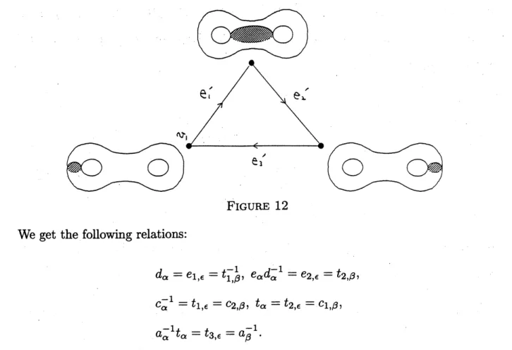
FIGURE 12 We get the following relations:

$d_{\alpha}=e_{1,\epsilon}=t_{1,\beta}^{-1},$ $e\alpha d_{\alpha}^{-1}=e2,\epsilon t2=,\beta$,

$c_{\alpha}^{-1}=t_{1,\epsilon}=c_{2,\beta},$ $t_{\alpha}=t_{2,\epsilon 1,\beta}=C$, $a_{\alpha}^{-1}t_{\alpha}=t_{3,\epsilon}=a^{-1}\beta$

.

To get the relations induced by (4),

we

need to give a presentation of$g_{\partial\tau_{1}}$ and $g_{\partial\tau_{2}}$.

Let $e_{1}^{\prime/;},$$e_{2},$ $e_{3}$ be the edgesof

$\partial\tau_{1}$ indicatedinFigure 12. We choose asequence$g_{1},$ $g_{2},$ $g_{3}$

of the elements of$\mathcal{H}_{2}$ corresponding to these edges. The element $d_{\gamma}$ of$G_{\sigma_{1}}$ satisfies $v_{1}d_{\gamma}$ $=t(e_{1})$, and $b_{\alpha}\in G_{v_{1}}$ satisfies $eb_{\alpha}=e_{1}’$, therefore,

we

choose $g_{1}=d_{\gamma}b_{\alpha}$

.

The element

$b_{\alpha}^{-1}$ of_{$G_{v_{1}}$} satisfies $eb_{\alpha}^{-1}=e_{2}’g_{1}-1$, therefore, we choose $g_{2}=d_{\gamma}b_{\alpha}^{-1}$

.

The element $b_{\alpha}$ of

$G_{v_{1}}$ satisfies $eb_{\alpha}=e_{2}’(g_{2}g1)-1$, therefore,

we

choose $g_{3}=d_{\gamma}b_{\alpha}$

.

The element $g_{3}g_{2}g_{1}$ is

in $G_{v}$, namely

we can

check $g_{3}g_{2}g_{1}=c_{\alpha}a_{\alpha}^{-1}d_{\alpha}e_{\alpha}$

.

Hence we get the following relation:

$d_{\gamma}b_{\alpha\gamma}db_{\alpha\gamma\alpha}^{-}1db\alpha=c_{\alpha\alpha}a^{-1}de\alpha$

.

Let $e_{1}$”, $e_{2}$”, $e_{3}$

” _{be the edges of}$\partial\tau_{2}$ indicated in Figure 13. By the same manner,

we get the following relation:

$d_{\gamma}=r_{\beta}^{-1}$

.

(13)

FIGURE 13

Tietzetransformations [MKS;

_{\S 1.5]}

to thispresentation, thenweobtain thepresentation

given in Theorem 1.

4. THE SURJECTION FROM $\mathcal{H}_{2}$ TO $GL(2, \mathbb{Z})$

There is a natural surjection from $\mathcal{H}_{2}$ to the outer automorphism group of the

free group ofrank 2, Out$(F_{2})$, which is defined by the action of the elements of

$\mathcal{H}_{2}$ on the

fundamentalgroup of the handle body of genus 2. _{For the sake of check the}presentation

given in Theorem 1, we show _{this result with using this} presentation. The group

Out$(F_{2})$ is naturally identified with $GL(2, \mathbb{Z})$ (see [MKS; p.169]). The group _{$GL(2, \mathbb{Z})$}

is generated by $R_{1},$ $R_{2},$ $R_{3}$:

$R_{1}=,$

_{$R_{2}=,$}

_{$R_{3}=$}

,

and the following is the set of relations between them which defines $GL(2, \mathbb{Z})$:

$R_{1}^{2}=R^{2}2=R^{2}3=E$,

$(R_{1}R_{2})^{3}=(R1R3)^{2}=Z$, $Z^{2}=E$_,

where

(14)

(see [CM; Chapter 7]).

A homomorphism $\psi$ from $\mathcal{H}_{2}$ to $GL(2, \mathbb{Z})$ defines by:

$a,$$c,t\mapsto E$,

$b\mapsto R_{1}R_{3}R_{2}R_{1}$, $d-R_{3}$,

$e-R_{1}R_{3}R_{1}R_{3}(=^{z)},$ $f\mapsto R_{1}R_{3}R1R_{3}R_{1}$,

isa naturalsurjection. Ahomomorphism $\phi$from$GL(2, \mathbb{Z})$ to$\mathcal{H}_{2}$definedby considering

natural identification of (once punctured torus) $\cross[0,1]$ with $H_{2}$ :

$R_{1}\mapsto fe$,

$R_{2}\mapsto d^{-1}ac^{-}1fbf$, $R_{3}-d^{-1}aC^{-1}$,

is

a

injection and satisfies.$\psi\circ\emptyset=idcL(2,\mathbb{Z})$

.

The above two facts

are

verified by using

the representation of$\mathcal{H}_{2}$ given

as

aTheorem 1.

Problem. A injection $\phi$ from $GL(2, \mathbb{Z})$ to $\mathcal{H}_{2}$ , which satisfies

$\psi\circ\emptyset=id_{GL(2},\mathbb{Z}$₎ is not

unique. Is it unique up to conjugation ?

REFERENCES

[Bi] J.S. Birman, Mapping class groups and their rerationships to braid groups, Comm. Pure Appl. Math. 22 (1969), 213-238.

[Br] K.S. Brown, Presentations

_for

groups

acting

on

simply-connected complexes,

Jour. Pure and Appl. Alg. 32 (1984), 1-10.

[CM] H.S.M. CoxeterandW.O.J.Moser, Generatorsand rerations

for

discretegroups, Ergebnisse der

mathematik

und ihrer grenzgebiete, band 14, Springer, 1972.

[Ha] A.E. Hatcher, A proof

_of

the Smale Conjecture, $Diff(S^{3})\simeq O(4)$, Ann. of

(15)

[J] K. Johannson, Topology and combinatorics

_of

3-manifolds, Lecture notes in math. 1599, Springer, 1995.

[K] R.Kramer, The twistgroup

_of

an orientable cube-with-two-handles is not finitely

generated, preprint.

[MKS] W. Magnus, A. Karras, D. Solitar, Combinatorial group theory, Interscience,

New York, 1966.

[S] S. Suzuki, On homeomorphisms

_of

a 3-dimensional handlebody, Canad. J. Math.

29 (1977), 111-124.

DEPARTMENT OF MATHEMATICS FACULTY oF SCIENCE AND ENGINEERING SAGA UNIVERSITY

SAGA, 840 JAPAN