Concurrent Programming
in
Linear Logic
Naoki Kobayashi
Toshihiro Shimizu
koba@is.s.u-tokyo.ac.jp
shimizu@is.s.u-tokyo.ac.jp
Akinori Yonezawa
yonezawa@is.s.u-tokyo.ac.jp
Department
of
lnformation
Science
University
of Tokyo
7-3-1
Hongo, Bunkyo-ku, Tokyo,
113
Japan
Abstract
HACL is a novel asynchronous concurrent programming language developed
based on linear logic. It provides fruitful mechanisms for concurrent
program-ming including higher-order concurrency and an elegant $\mathrm{M}\mathrm{L}$-style type system.
Although HACL provides only a small set ofprimitive constructs, various
con-structs forcommunicationand synchronization between processes are definable in
termsof primitive asynchronous message passing and higher-order processes. In
this paper, we demonstrate the power of HACLbyshowing severalprogramming
examples. For readers who are not familiar with linear logic and concurrent linear
logic programming, we also give abrief introduction to the logical background
ofHACL.
1
Introduction
We developed a novel typed, higher-order, concurrent programming language called
HA CL based on ahigher-orderextension of$\mathrm{A}\mathrm{C}\mathrm{L}[3][2]$
.
ACL is a variant of linear logicprogramming, whose operational semantics is described in terms ofbottom-up search
for a cut-free proof in linear logic. ACL naturally models concurrent computation
based
on
asynchronous message passing, while traditional concurrent logicprogram-ming languages model stream-based communication. In the $\mathrm{P}^{\mathrm{r}\mathrm{e}\mathrm{V}\mathrm{i}\mathrm{o}\mathrm{u}\mathrm{S}}.\mathrm{P}^{\mathrm{a}}\mathrm{p}\mathrm{e}\mathrm{r}\mathrm{S}[3][2]$
,
wehave shownmost of computational models for asynchronous concurrent computation,
includingactor models, Linda, concurrent constraint programming,and asynchronous
counterpart of CCS and $\pi$-calculus,
can
be naturally embedded in ACL. The power of ACL can be further strengthened by replacing the underlying logic withhigher-orderlinear logic. The resulting framework, Higher-Order $\mathrm{A}\mathrm{C}\mathrm{L}[5]$ (in short, HACL),
by other processes, communicationinterfaces, and functions. HACL is also equipped
with an elegant $\mathrm{M}\mathrm{L}$-style type system, hence the type inference system infers the
most general types for untyped programs, and ensures that any well-typed program
never causes type mismatch error at run-time.
The purpose of this paper is to demonstrate the power of HACL by showing
several
program.ming
examples. Higher-order processes allow us to define a largeprocess by composing smaller subprocesses, by which improving the modularity and code reuse ofconcurrent programs, and are also useful for making topologies between multiple processes. Therefore, various constructs for concurrent programming, which are introduced as primitives in an $ad$ hoc manner in many concurrent programming
languages, can be defined using higher-order processes. HACL also allows
object-oriented style programming, as is shown in [4]. We believe that HACL can be used
not onlyas aspecificconcurrent programming language, butalso as acommon vehicle
to design novel, clean and powerful $\mathrm{c}\mathrm{o}\mathrm{n}\dot{\mathrm{c}}$
urrent programming languages, to develop
program analysis techniques for concurrent programming languages, and to discuss
efficient implementation techniques.
Prototype interpreter of HACL and examples given in this paper are availablevia anonymous ftp from $\mathrm{c}\dot{\mathrm{a}}\mathrm{m}\mathrm{i}\mathrm{l}\mathrm{l}\mathrm{e}$
.
is.$\mathrm{s}.\mathrm{u}$-tokyo.$\mathrm{a}\mathrm{c}$
.
jp: $\mathrm{p}\mathrm{u}\mathrm{b}/\mathrm{h}\mathrm{a}\mathrm{c}\mathrm{l}$.
2
Overview
of Higher-Order ACL
This section informally overviews the syntax and operational semantics of
higher-order ACL. For the concrete definitions, please refer to $[5][4]$
.
For readers who arenot familiar with linear logic and concurrent linear logic programming, we attach a brief introduction to both linear logic and its connection with concurrentcomputation in Appendix.
Asin thefirst-order$\mathrm{A}\mathrm{C}\mathrm{L}[3][2]$
,
computationin Higher-order ACL (in short, HACL)is described in terms of bottom-up proof search in Girard’s (higher-order) linear
$\mathrm{l}\mathrm{o}\mathrm{g}\mathrm{i}\mathrm{c}[1]$
.
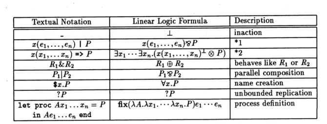
Each formula of (a fragment of) higher-order linear logic is viewed as aprocess, while each sequent, a multiset offormulas, is regarded as a certain state of
the entire processes. A message is represented by an atomic formula, whose
predi-cate is called a message predicate. The whole syntax of HACL process expressions is summarized in Figure 2. The first column shows textual notations for process expres-sions. The second column shows corresponding formulas of linear logic. In the figure,
$x$ is ranged over variables, $P$ over process expressions, and $R$ over process
expres-sions of the form $x(x_{1}, \ldots, xn)=\rangle P$
.
A behavior ofeach $\mathrm{p}\mathrm{r}o$cess is naturally derivedfrom inference rules of linear logic. For example, from the inference shown in the
Figure 1, we can regard a formula$\exists x_{1}\cdots\exists x_{n}.(X(x_{1}, \ldots, Xn)^{\perp}\otimes P)$ as a process which
receives a message $x(v_{1}, \ldots, v_{n})$ and then behaves like $P[v_{1}/x_{1}, \ldots, v_{n}/x_{n}]^{1}$
.
Messagepredicates are created by the
$(V,
in linear logic notation) operator. $x.P creates amessage predicate and binds $x$ to it in $P$. A choice $(\mathrm{m}(\mathrm{x})=\rangle \mathrm{p})\ (\mathrm{n}(\mathrm{X})=\rangle \mathrm{Q})$ either
re-ceives a message$\mathrm{m}(\mathrm{v})$ and becomes $\mathrm{P}[\mathrm{v}/\mathrm{x}]$, or receives amessage $\mathrm{n}(\mathrm{v})$ and becomes
$\frac{\vdash x(v_{1},..\cdot.\cdot..\cdot’.v_{n}),x(v_{1},...\cdot.’v_{n})^{\perp}.\vdash P[v_{1}/x_{1},..\cdot.\cdot.’.v_{n}/xn],\mathrm{r}}{\frac{\vdash x(v_{1},,v_{n})^{\perp}\otimes P[v1/x_{1},..,v_{n}/x_{n}],x(v_{1},.,v_{n}),\Gamma}{\vdash\exists x_{1}\exists x_{n}.(x(x_{1},.,x_{n})^{\perp}\otimes P),x(v1,.,v_{n}),\mathrm{r}}\exists}\otimes$
Figure 1: Inference corresponding to Message Reception
$\mathrm{Q}[\mathrm{v}/\mathrm{x}]$
.
A proc statement defines a$\mathrm{r}\mathrm{e}\acute{\mathrm{c}}\mathrm{u}\mathrm{r}\mathrm{S}\mathrm{i}\mathrm{v}\mathrm{e}$process just as a funstatement defines a recursive function in $\mathrm{M}\mathrm{L}$
.
For example,proc forwarder $\mathrm{m}\mathrm{n}=\mathrm{m}\mathrm{x}=>\mathrm{n}\mathrm{x}$; $\mathrm{v}\mathrm{a}l$forwarder
$=proc:(’ a->\mathit{0})->(’ \mathrm{a}->\mathit{0})_{->}\mathit{0}$
defines forwarder as a process which takes twomessage predicates $\mathrm{m}$ and $\mathrm{n}$ as
argu-ments, and receives a value of$\mathrm{x}$ via a message $\mathrm{m}$ and sends it via a message $\mathrm{n}$
.
Theline printed in slanted $\psi \mathrm{y}\mathrm{l}\mathrm{e}$ is the system’s output. It indicates that forwarder has
the following type:
$\forall\alpha.((\alphaarrow \mathit{0})arrow(\alphaarrow \mathit{0})arrow \mathit{0})$,
where $\mathit{0}$ is the type for processes or messages. Therefore, the type of forwarder
implies that it
takes
two message predicates, $\mathrm{w}\mathrm{h}\mathrm{i}\mathrm{C}_{\backslash }\mathrm{h}$should take an argument of thesame
type.2
A process point is defined in HACL as follows:
proc point ($\mathrm{x}$, y) (getx, gety, set) $=$
getx(reply) $=\rangle$
(reply(x) $|$ point
$(\mathrm{x},\mathrm{y})(\mathrm{g}.\mathrm{e}\mathrm{t}\mathrm{x}$,gety,set))
&gety(reply) $=\rangle$
(reply (y)
1
point$(\mathrm{x},\mathrm{y})$ (getx,gety,set))& set (newx,newy, $\mathrm{a}\mathrm{c}\mathrm{k}$)$=>$
(ack ()
1
point(newx,newy) (getx,gety,set));$\mathrm{v}\mathrm{a}l$poin
$t=_{P^{roc}}:’ \mathrm{a}*’ b_{->}((’ a_{->O})_{-}>\mathit{0})*((’ \mathrm{a}_{->O})->\mathit{0})*(’ \mathrm{a}*’ b_{->)->}o.\mathit{0}$
The process point has two internal state variables $\mathrm{x}$ and
$\mathrm{y}$
,
and is parameterized bymessage predicates getx, gety, and set. If it receives a getx message, it sends the
value of $\mathrm{x}$ to the reply destination reply. If it receives a set message, it sends an
acknowledgement message ack$()$, and changes values of$\mathrm{x}$ and
$\mathrm{y}$ to newx and newy.
The following expression creates anewpoint process, and sends toit agetxmessage.
$getx. $gety.$set.
(point(1.0, 2.0) (getx,gety,set) $|$ $reply. (getx (reply) $|$ reply$(\mathrm{x})=>$
.
$*_{1}\ldots$ sends a message $x(e_{1}, \ldots , e_{n})$, and then behaves like $P$
$*_{2}\ldots$ receives a message $x$($e_{1,\ldots,}$e), and then behaves like $P[e_{1}/x_{1}, \ldots,e_{n}/x_{n}]$
Figure 2: Syntax of HACL process expressions
3
Programming in
HACL
This section demonstrates the $\mathrm{p}\mathrm{o}\mathrm{w}^{\backslash }\mathrm{e}\mathrm{r}$ofHACL, by showing several examples of
con-current
programming
in HACL. In HACL, processes can be parameterized by otherprocesses and interfaces (message predicates), just asfunctions can beparameterized
by other functions in functional programming. This dramatically improves the mod-ularity and code reuse of concurrent programs. We also show that HACL extended with records naturally allows $\mathrm{c}\mathrm{o}\mathrm{n}\mathrm{c}\mathrm{u}\backslash$rrent object-oriented style
programming.
3.1
Object-Oriented
Style
Programming
In the definition ofpoint process in the previous section, readers might have noticed
that it is very cumbersome to separately create getx, gety, and set message
predi-cates, and to remember in which order they should be applied to the point process.
In order to overcome this problem, it is very natural to introduce records, and put the three message predicates together in a record:
proc point ($\mathrm{x}$, y) self $=$
#getx self (reply) $=\rangle$ ($\mathrm{r}\mathrm{e}\mathrm{p}\mathrm{l}\mathrm{y}(\mathrm{x})|$ point(x.y) self )
& #gety self (reply) $=\rangle$ ($\mathrm{r}\mathrm{e}\mathrm{p}\mathrm{l}\mathrm{y}(\mathrm{y})|$ point(x,y) self )
&#set self (newx,newy)$=>$ (point(newx,newy) self );
$\mathrm{v}al_{P}o.int=proc:’ a*’ b->’ C::\mathrm{t}getx:(’ \mathrm{a}->\acute{o})->\mathit{0},$ $g\mathrm{e}ty:(’ b->\mathit{0})->\mathit{0},$ $set:’ \mathrm{a}*’ b-$
$>\mathit{0}\}->O$
$\#\langle \mathrm{f}\mathrm{i}\mathrm{e}\mathrm{l}\mathrm{d}$-name) is an operator for field extraction. The resulting process definition just
looks like the definition of concurrent $\mathrm{o}\mathrm{b}\mathrm{j}\mathrm{e}\mathrm{c}\mathrm{t}\mathrm{S}[10]$
.
self, which is a record consistingof at least three fields getx, gety, and set, can be considered as an
identifier
ofordinary object-oriented languages. The typeinference is basedon Ohori’s algorithm
for polymorphic record $\mathrm{c}\mathrm{a}\mathrm{l}\mathrm{C}\mathrm{u}\mathrm{l}\mathrm{u}\mathrm{S}[6]$
.
The inferred type indicates that point takes apair of values of type $\alpha$ and $\beta$ as its first argument, and a record of type {getx :
$(\alphaarrow \mathit{0})arrow \mathit{0}$,gety: $(\betaarrow \mathit{0})arrow \mathit{0}$,set: $\alpha\cross\betaarrow \mathit{0},$
$\ldots$
}
as its second argument self.The following is an expression for creating a new point object and sends to it a
message getx.
$id. (point (1.0, 2.0) id $|$ $reply. (#getx id reply $|$ reply$(\mathrm{x})=>$
.
.
.)Ifaprogrammer wants to ensure that messages except for getx, gety, and set are
neversent to the point object, he can explicitly attach the following type constraints
on self:
proc point ($\mathrm{X}$, y) (self:{getx: ’$\mathrm{a}$, gety: ’
$\mathrm{b}$, set: ’$\mathrm{c}\}$) $=$
#getx self (reply) $=\rangle$ ($\mathrm{r}\mathrm{e}\mathrm{p}\mathrm{l}\mathrm{y}(\mathrm{x})|$ point(x,y) self )
& #gety self (reply) $=\rangle$ ($\mathrm{r}\mathrm{e}\mathrm{p}\mathrm{l}\mathrm{y}(\mathrm{y})$ $|$ point(x,y) self )
&#set self (newx,newy)$=>$ (point(newx,newy) self );
$\mathrm{v}\mathrm{a}l$point
$=proc:’ \mathrm{a}*’ b->\{g\mathrm{e}t\mathrm{x}:(’ a->\mathit{0})->\mathit{0}, gety:(’ b->\mathit{0})->0, Set:’ \mathrm{a}*’ b_{-}>\mathit{0}\}-$
$>O$
Then, sending a message other than getx, gety and set is statically detected as an
invalid field extraction from the record self.
Based on these observations, we can easily construct a typed concurrent object-oriented programming language with inheritance and method overriding on top of HACL. By the type system of HACL, all message not understood errors can be statically detected at type-checking phase.[4]
3.2
Synchronization and
Sequencing
between Processes
It is often important to write synchronization or serialization of execution of pro-cesses. Constructs for such purposes can bedefined using higher-order processes. For example, consider thefollowing process seq:
proc seq $(\mathrm{p}1, \mathrm{p}2)=$ $token. (pl(token) $|$ token$()=>$ p2()); $\mathrm{v}\mathrm{a}l$
$seq=p\mathrm{r}oc:((\mathrm{u}\mathrm{n}it->\mathit{0})->\mathit{0})*(\mathrm{u}nit->\mathit{0})->\mathit{0}$
seq (soutput$(^{\mathrm{t}}’ \mathrm{h}\mathrm{e}110’\dagger)$ , fn $()=>\mathrm{o}\mathrm{u}\mathrm{t}\mathrm{p}\mathrm{u}\mathrm{t}(^{11}\mathrm{w}\mathrm{o}\mathrm{r}\mathrm{l}\mathrm{d}\backslash \mathrm{n}\dagger|)$);
hello world
seq$(\mathrm{p}1, \mathrm{p}2)$ executes a process pl(token) at first, and p2$()$ is invoked only when
the process pl sends a message token$()$
.
soutput is a built-in process which takesa string $s$ and a message predicate $m$ as an
argume.
$\mathrm{n}\mathrm{t}$.
It displays $.$$\mathrm{t}$he string
$s$, and
then sends the message $m()$.
It is also easy to write processes for realizing broadcast, barrier synchronization,
etc. For example, the followingprocess make-group takes amessage predicate $\mathrm{m}$ and
a list ofprocesses procs as arguments. Sending a message $\mathrm{m}(\mathrm{x})$ from the externals
local
proc $\dot{\mathrm{b}}$roadcast
$\mathrm{x}$ ns $=$
case ns of nil $=>$
$|\mathrm{n}$: :$\mathrm{n}\mathrm{s}’=\rangle$ ($\mathrm{n}(\mathrm{x})|$ broadcast $\mathrm{x}\mathrm{n}8’$)
in
proc broadcaster $\mathrm{m}$ ns $=$
$\mathrm{m}(\mathrm{x})=>$ (broadcast(1. $\mathrm{n}\mathrm{s})|$ broadcaster $\mathrm{m}\mathrm{n}\mathrm{s}$)
end local
proc parapp procs ms $=$
case procs of
nil $=>$
$-$
$|\mathrm{p}\mathrm{r}$::procs’ $=>$ (case ms of $\mathrm{m}$: :$\mathrm{m}\mathrm{s}’=>(\mathrm{p}\mathrm{r}(\mathrm{m})|$ parapp procs’ $\mathrm{m}\mathrm{s}’)$) in
proc make-group $\mathrm{m}$ procs $=$
let
val $\mathrm{g}\mathrm{s}\mathrm{i}\mathrm{z}.\mathrm{e}$
.
$=$ length(procs)
in
$\mathrm{m}\mathrm{a}\mathrm{k}\mathrm{e}_{-,-}\mathrm{m}\mathrm{p}\mathrm{r}\mathrm{e}\mathrm{d}_{-\mathrm{S}}1\mathrm{i}\mathrm{t}$ (gsize. fn $\mathrm{x}=>$ (broadcaster $\mathrm{m}\mathrm{x}|$ parapp procs
$\mathrm{x})$)
end
end
3.3
Higher-Order
Processes for
Making Topologies
between
Processes
Higher-orderprocesses in HACL are especially useful for making topologies between
processes. For example, consider the following higher-order process linear:
proc linear procs left right $=$
case procs of
nil $=>$
$|\mathrm{p}\mathrm{r}$: :nil $=>\mathrm{p}\mathrm{r}$(left, right)
$|\mathrm{p}\mathrm{r}$: :procs2 $=\rangle$ $link. (
$\mathrm{p}\mathrm{r}$(left, link)
$|$ linear procs2 link right);
$\mathrm{v}alli\mathrm{n}ear=p\mathrm{r}oc:((’ a->\mathit{0})*(’ a->\mathit{0})->\mathit{0})$ list-$>(’ a->\mathit{0})->’(a->\mathit{0})->\mathit{0}$
We use the notation of ML for the case statement and list expressions. The
higher-order process linear takes a list of processes procs as the first argument, and
con-nects themin a lineartopology. Aringstructurecan be constructedby just assigning
the same message predicate to the left and right of linear process.
$\mathrm{p}\dot{\mathrm{r}}$oc ring procs $=$ $m.(linear procs $\mathrm{m}\mathrm{m}$); $\mathrm{v}al$$ring=p\mathrm{r}oc:((’ \mathrm{a}->\mathit{0})^{*}(’ a->\mathit{0})->\mathit{0})$ $list->\mathit{0}$ The dining philosopher problem can $\dot{\mathrm{b}}\mathrm{e}$
described by defining a behavior of each
$*9f\approx \mathrm{f}\mathrm{f}\mathrm{l}\mathrm{g}\tau\epsilon \mathrm{P}_{\mathrm{M}}\mathrm{t}\mathrm{y})\emptyset \mathrm{f}\mathrm{f}\mathrm{l}\epsilon*\mathrm{g}\ovalbox{\tt\small REJECT} \mathrm{b}f\underline{\wedge}@\mathrm{f}\mathrm{f}\mathrm{i}$ $T$$\hslash 6$
.
$[\ovalbox{\tt\small REJECT}\not\equiv 3\cdot 1]$ 2
(1) $\mathrm{v}\in \mathrm{V}_{\mathrm{t}}$op(PN$(\mathrm{x})$ )$\mathrm{g}6l\mathrm{f}$, label($\delta$
*PM
$(,\mathrm{x})\Leftrightarrow \mathrm{P}\mathrm{M}\langle \mathrm{y}$)$\langle \mathrm{v}\rangle)=$ label
1
$\delta$fPM
$\mathrm{t}\mathrm{x}$) $(\mathrm{v}))$.
{$2\rangle \mathrm{v}\in \mathrm{V}_{\mathrm{b}\mathrm{o}\mathrm{t}}$ (PM(y) )$r_{J}\mathrm{e}\iota \mathrm{f}$, label($\delta$
*PM
(x)$\mathrm{e}\mathrm{P}u\langle \mathrm{y}$)$(\mathrm{v}))=$ label
$\mathrm{t}\delta \mathrm{s}_{\mathrm{P}_{\mathrm{b}\mathrm{t}}\mathrm{t}\mathrm{y}\rangle}(\mathrm{v}))$
.
( $\ovalbox{\tt\small REJECT}$ff,#$\Re\rangle$
I
$\theta_{\mathrm{P}}\not\in 3$.
2 $\omega^{-}\mathrm{F}\vee \mathfrak{M}0\ovalbox{\tt\small REJECT}\gtrless$ ] $\mathrm{z}\xi \mathrm{x}\emptyset\lrcorner_{\mathrm{i}}\#\epsilon\epsilon \mathrm{y}\omega^{-}\mathrm{r}*9\#\backslash \not\in$ae
$\mathrm{b}\gamma_{\simeq}2r\lambda\overline{\pi}\overline{\mathcal{T}}-\text{フ^{}\mathrm{o}}$,$T^{r_{Jb\mathrm{t}}}$
.
i) $\mathrm{Q}_{1}(\mathrm{z})=\mathrm{n}_{2}(\mathrm{Z})--_{2\mathrm{m}}$,
ii) $\mathrm{z}[(1,1\rangle , (\mathrm{m}, 2\mathrm{m})]=\mathrm{x}[\mathrm{t}1,1),$ $(\mathrm{m}, 2\mathrm{m})]$ ,
iii) $\mathrm{z}[(\mathrm{m}+1,1\rangle , (2\mathrm{m}, 2\mathrm{m})]=\mathrm{y}[\mathrm{l}\mathrm{m}+1,1)$ ,$\mathrm{t}2\mathrm{m},$$2\mathrm{m})]$
$\mathcal{E}T6$
.
$arrow\veearrow \mathrm{T}^{\backslash }\vee,$ mM5-ト$\Rightarrow*\grave{[}\mathrm{R}\mathrm{o}^{\sim}\mathrm{g}\beta f\mathrm{g}$ $\mathrm{v}_{0}$ $k\mathfrak{B}\#$.
a
$T6$ $\mathrm{P}_{\mathrm{M}}(\mathrm{x})\mathrm{e}$PM$\mathrm{t}\mathrm{y}$) $\downarrow \mathcal{O}$)$\mathrm{a}\Re_{\grave{1}}\underline{langle}$ $\epsilon\Rightarrow\overline{\mathrm{X}}6$ :$\underline{(^{\sim}1}r1\mathrm{v}:=\mathrm{v}_{0}\epsilon h^{\backslash }<$
.
$\cap\underline{2}$ $\mathrm{b}\mathrm{b}*$ $\delta\star(\mathrm{v})_{-}-\{\mathrm{V}’\}\gamma x\epsilon^{\mathrm{m}}\epsilon \mathrm{p}|\mathrm{g}_{\backslash }.\iota^{r}$$’\in \mathrm{V}\{\mathrm{p}_{\mathrm{N}}(\mathrm{X})\ominus \mathrm{p}_{\mathrm{M}(}\mathrm{y}))\delta^{\mathrm{i}^{\backslash }}T\neq\not\in\tau$
6&6
$l\mathrm{f}$, $\mathrm{v}:=\mathrm{v}$’8
$\mathrm{k}^{\backslash }1\backslash \tau_{\mathrm{c}}|\gamma 2\epsilon\ovalbox{\tt\small REJECT} \mathfrak{y}\grave{x}\underline{\mathrm{B}}\tau$.
$\not\in$ \={o} $\tau\cdot r_{J}\mathrm{t}\gamma nl\mathrm{f}$.
$,$
$\not\in$A$\mathrm{Y}6$
.
$\ovalbox{\tt\small REJECT}\not\equiv 3$
.
13:
$|?$ , $\ovalbox{\tt\small REJECT}\Re \mathrm{v}\emptyset \mathrm{f}\mathrm{F}\emptyset’\yen_{\backslash }p_{t}\int\emptyset\backslash ^{*}$ $( arrow \mathrm{Y}\mathrm{x}\Phi^{\Rightarrow}\mathrm{s}+\geqq*if8\mathrm{o}^{rightarrow 5_{\backslash }}\mathrm{B}\mathbb{R}i.\mathrm{r} \mathrm{v}_{1\{}\mathrm{b}\mathrm{b}\langle l\mathrm{f} \mathrm{u}_{\mathrm{J}}\mathit{0})\prod \mathrm{r}\hslash$ $p\backslash *(-\not\in \mathrm{i}_{\backslash r’\cdot\backslash }\mathrm{a}g\mathrm{g}T\delta)\mathrm{M}\emptyset \mathrm{z}$ -k$\emptyset\hslash 6\mathrm{L}(\mathrm{m}\mathrm{I}\mathrm{f}\mathrm{f}\mathrm{i}\Phi\Phi\overline{j\mathrm{E}}\mathrm{X}\mathrm{I}\mathrm{E}\mathrm{g}$ $a\equiv \text{ト}\Rightarrow \mathrm{f}\mathrm{f}\mathrm{i}\ovalbox{\tt\small REJECT} \mathrm{p}_{\kappa()}\mathrm{Z}$&ffl;\Re $\tau$a
$arrow\vee\succeq f\mathrm{g}$$\mathrm{E}\int \mathrm{j}6\theta^{1}$
.
$l^{\backslash }A4_{\mathrm{i}}b_{-\lambda}^{arrow}\mathfrak{y}$ , $\mathrm{z}\in \mathrm{T}\mathrm{t}\mathrm{M}$)$p\backslash \yen^{p_{1}}\backslash \backslash t\mathrm{t}\gamma_{\simeq}p\backslash ^{*}$, $arrowarrow n\mathrm{t}\mathrm{f}$’ $\mathrm{T}\mathrm{l}\mathrm{M}$)$–\mathrm{T}_{1}r_{\mathrm{a}^{\backslash }}\epsilon\ovalbox{\tt\small REJECT} \mathrm{t}V\omega \mathfrak{R}\overline{i\mathrm{E}}\iota_{\sim \mathrm{B}}^{\wedge}T$ \S $(\mathrm{z}\not\in \mathrm{T}_{1}f_{-\dot{|}}^{\sim\pm}grightarrow)$ $\square$$\mathrm{r}\mathrm{m}3\cdot 1]\mathrm{R}\mathfrak{B}_{\mathrm{c}}^{*}\mathrm{g}^{\tau}\not\in\downarrow \mathrm{r}\xi rarrow\emptyset\vee$
’ $arrow\veearrow T\vee\cdot \mathrm{t}\mathrm{f}$
ffi7
,$.\mathit{9}_{\backslash \backslash }\mathrm{V}8\not\in\emptyset \text{フ^{}p}-\backslash \cdot$$\backslash \triangleright 1\mathrm{a}\mathrm{L}^{r}\mathrm{e}1\{\iota^{*})\mathrm{g}\subset,c\mathrm{B}|\mathrm{J}\mathrm{b}\gamma_{\mathrm{d}\backslash }\backslash$) $1^{)}\mathrm{c}arrow \mathcal{E}l_{arrow}^{arrow}\tau$ \S . 2 $\backslash /\mathrm{A}\overline{\pi}\overline{\tau}-$フ$\circ$
x
$\mathcal{E}\mathrm{y}\mathrm{t}_{\vee}^{\sim}X\backslash \mathrm{f}\mathrm{Y}$ \S$\acute{\mathrm{x}}\mathrm{g}\mathrm{R}\equiv+a\Rightarrow \mathrm{E}\Re$PN$1\mathrm{x}$),PN(y)$p\backslash \not\in r\iota\epsilon\hslash$,...
$,$$\nwarrow r_{1}$,$\mathrm{u}_{1},\ldots$ ,$\mathrm{u}\mathrm{z}$,$\mathrm{v}_{2},\ldots$ ,$\mathrm{v}_{3},\mathrm{u}_{9}.,\ldots$ ,$\mathrm{u}_{4},\mathrm{v}_{4}$,...
,$\mathrm{v}\mathrm{s},$us,$\ldots$ ,$\mathrm{u}\epsilon,\mathrm{v}_{6},\ldots,\mathrm{v}-,\mathrm{u}_{7},\ldots,\mathrm{u}_{8},\mathrm{v}_{8}$
...
$\prime_{d^{\backslash }}$. $6L^{\mathrm{r}}\mathfrak{l}_{arrow}\wedge$ ,...
,$\mathrm{v}’ 1,\mathrm{u}_{3},$$\ldots,\mathrm{u}’ 2,$$\backslash ^{r}\mathrm{s},\ldots,\mathrm{V}’ 3,$$\mathrm{U}5,\ldots,\mathrm{u}’ 4,\mathrm{v}_{2}$ ,...
,$\tau^{\gamma}$’ $\mathrm{s},\mathrm{u}_{1},\ldots,\mathrm{u}’ 6,\mathrm{v}_{6},\ldots,\mathrm{V}’ 7,\mathrm{u}_{7},\ldots,\mathrm{u}’ 8,\mathrm{v}_{6}\ldots$ $\mathcal{E}\not\equiv<\sigma_{-}\star t\iota\delta 4_{\circ\emptyset 8\tau\S}(\mathrm{E}^{\backslash }2$ (a)$r_{J}6(y.\}_{\sim}^{\wedge}(\mathrm{b})e\sim*\#\mathrm{P}\backslash )$.
$-\vee\emptyset \mathcal{E}\mathrm{g}$.
$\mathrm{X}\emptyset \mathrm{k}-*9\epsilon \mathrm{y}\emptyset\uparrow$$\not\simeq’k^{\lambda}*\grave{)}\underline{\Phi}$
f#
$\llcorner f\underline{arrow}2tfi\backslash \overline{\pi}\overline{\mathcal{T}}-$フo $\mathrm{Z}t\approx \mathrm{x}_{\backslash }\iota \mathrm{b}T*;^{\backslash }\lambda\emptyset$A
$*\overline{\supset}^{\gamma.p}\mathrm{d}^{\backslash }\mathrm{X}\mathrm{E}\overline{\exists}+\mathrm{r}\Rightarrow \mathrm{f}\mathrm{f}_{L}\Re \mathrm{P}_{\mathrm{M}}\mathrm{t}\mathrm{Z}$)$\theta \mathrm{l}$ffl
$’$
ffi
$\mathrm{S}n$$6$
.
...
,$\mathrm{v}_{1},\mathrm{u}_{1},\ldots,\mathrm{u}’\epsilon,\mathrm{v}\iota,\ldots,\mathrm{v}_{5},\mathrm{u}_{5},\ldots,\mathrm{u}’ 4,\mathrm{v}_{2},\ldots,\mathrm{v}_{3},\mathrm{u}_{3},\ldots,\mathrm{u}’ 2,\mathrm{v}_{8}\ldots$$( \mathrm{E}2(\mathrm{c})4\sim\approx\oint \mathrm{e}\backslash )\square$
$[\mathrm{f}\mathrm{f}\mathrm{l} \ovalbox{\tt\small REJECT} 3.2 \sigma 2\ovalbox{\tt\small REJECT}^{\beta}\beta\sigma)\ovalbox{\tt\small REJECT} \mathrm{g}]$ $8\mathrm{E}6\delta\backslash \mathrm{t}\sim|arrow,$ $|\mathrm{V}(\mathrm{m})|=(2\mathrm{m}$I$\mathrm{m}T^{\backslash }b6$
.
$-x,$ $\mathrm{g}_{\mathrm{m}\underline{\rangle}1}\iota_{-\Re}^{\sim}$$\mathrm{b}T$ ,
$\mathrm{C}(\mathrm{m})=$ { $\mathrm{C}\mathrm{r}\mathrm{o}\mathrm{s}\mathrm{s}_{-}\mathrm{P}\mathrm{a}\mathrm{i}\mathrm{r}$(PN$1\mathrm{x}\rangle$ ) $|\exists \mathrm{x}\in \mathrm{V}\mathrm{l}\mathrm{m})$ [PM$(\mathrm{X})\iota \mathrm{f}\mathrm{M}\mathrm{o}_{\mathrm{X}_{-}\mathrm{b}}\emptyset$
$\mathrm{L}(\mathrm{m})\mathrm{f}\mathrm{f}\mathrm{i}\mathfrak{B}\Phi_{\hat{\mathrm{E}}^{\mathfrak{B}}}\mathrm{J}\mathrm{g}\mathrm{x}$
5-ト$\Rightarrow \mathrm{E}$ffl] }
8
$k^{\backslash }\mathrm{t}\mathrm{J}l\mathrm{f}$ ,$|\mathrm{C}(\mathrm{m})|\leqq$
$\mathrm{L}_{-}^{-}\mathrm{o}\Sigma$
$\llcorner \mathrm{e}[\mathrm{m}]/2_{\mathrm{J}}$
.
$\leqq$
$\{\mathrm{e}[\mathrm{m}]\mathrm{L}=0\Sigma\}\leqq 222\cdot \mathrm{e}[\mathrm{m}]$$p\backslash ;\mathfrak{X}\mathfrak{y}\mathrm{E}\cdot\supset$
.
$arrow\veearrow\vee l_{\sim}^{\wedge}$ , $\mathrm{e}[\mathrm{m}]=\mathrm{s}(2\mathrm{m}+2)\mathrm{L}\{2\mathrm{m}\rangle$$\mathrm{t}^{\mathrm{L}\mathrm{t}2\mathrm{m})}$,$\mathrm{S}$ tf$\mathrm{M}\emptyset\#\Phi$
ffiJ
$\ovalbox{\tt\small REJECT} \mathrm{f}\mathrm{f}\mathrm{l}\emptyset*\ovalbox{\tt\small REJECT}\Re$ , $\mathrm{t}$2 ク“$\text{フ}-$
フ $\mathrm{G}\mathrm{o}_{\mathrm{R}}^{\mathrm{m}_{\beta}}$
A
$k_{\dot{\mathfrak{Q}}}^{\Delta}$」, $\mathrm{a}\ovalbox{\tt\small REJECT}_{\square ^{\hslash\backslash ^{\backslash }}}^{\mathrm{A}}\backslash$ ,
$\epsilon n\epsilon n\mathrm{v}\mathrm{t}\mathrm{G}$), $\mathrm{E}(\mathrm{G})\emptyset\epsilon \mathrm{g},$ $\Leftrightarrow \mathrm{V}\in \mathrm{V}(\mathrm{G})\iota_{-}^{\sim}\Re \mathrm{b}T$ , $\delta \mathrm{s}_{\mathrm{G}(_{\mathrm{V}})}=\{\mathrm{v}’\in \mathrm{v}\langle \mathrm{G}\}|1\mathrm{v},\backslash \gamma’)\in \mathrm{E}\mathrm{t}\mathrm{G})\}\epsilon\not\in\ovalbox{\tt\small REJECT} T\epsilon$
.
($\mathrm{a}\mathrm{c}\mathrm{k}()$ $|$ point$(\mathrm{x}+\mathrm{d}\mathrm{x}+0.0,$ $\mathrm{y}\star \mathrm{d}\mathrm{y}+0.0)$ self );
$\mathrm{v}al$point$=p\mathrm{r}oc:real^{*}real->’ \mathrm{a}::\{get\mathrm{X}:(\mathrm{r}ea\iota_{-}>\mathit{0})_{->}\mathit{0},$ $get_{X}:(real->\mathit{0})->\mathit{0},$$mo\mathrm{V}e.re\mathrm{a}\mathit{1}*era\mathit{1}*(\mathrm{u}\mathrm{n}it$
$>\mathit{0})->\mathit{0}\}->O$
We can define a rectangle process by composing two point processes as follows.
local
proc rectangle’ $(\mathrm{p}1, \mathrm{p}2)$ self $–$
#getcx self (reply) $=>$
($m. (#getx pl $\mathrm{m}|\mathrm{m}(\mathrm{x}\mathrm{l})-->$ (#getx p2 $\mathrm{m}|\mathrm{m}(\mathrm{x}2)=>$
(reply$((\mathrm{x}1+\mathrm{X}2)/2.0)$ $|$ rectangle’ $(\mathrm{p}1,$ $\mathrm{p}2)$ self )$)))$
& #getcy self (reply) $=>$
($m. (#gety pl $\mathrm{m}|$ m(yl)$=>$ (#gety p2 $\mathrm{m}|\mathrm{m}(\mathrm{y}2)=>$
(reply$((\mathrm{y}\mathrm{l}+\mathrm{y}2)/2.0)$ $|$ rectangle’ $(\mathrm{p}1,$ $\mathrm{p}2)$ self )$)))$ & #move self $(\mathrm{d}\mathrm{x}, \mathrm{d}\mathrm{y}, \mathrm{a}\mathrm{c}\mathrm{k})=>$
($ack2. (#move pl ($\mathrm{d}\mathrm{x},\mathrm{d}\mathrm{y}$,ack2)
$|$ ack2$()=>$($\#\mathrm{m}\mathrm{o}\mathrm{v}\mathrm{e}$ p2 $(\mathrm{d}\mathrm{x},\mathrm{d}\mathrm{y},\mathrm{a}\mathrm{C}\mathrm{k})$ $|$ rectangle2 $(\mathrm{p}1,$ $\mathrm{p}2)$ self )
in
proc rectangle (pointl, point2) self $=$
$idl. $id2. (point1 idl $|$ point2 id2 $|$ rectangle’ $(\mathrm{i}\mathrm{d}\mathrm{l},$ $\mathrm{i}\mathrm{d}2)$ self )
end;
A particular instance of rectangle process is created by instantiating pl and p2 to point processes as follows:
proc new-rectangle $(\mathrm{x}1, \mathrm{y}1, \mathrm{x}2, \mathrm{y}2)$ self $=$
rectangle (point$(\mathrm{x}1,$ $\mathrm{y}1)$ , point$(\mathrm{x}2,$ $\mathrm{y}2)$) self;
$\mathrm{v}\mathrm{a}l\mathrm{n}$ew-rectangle$=proc:re\mathrm{a}l*real*real*\mathrm{r}eal->’ \mathrm{a}::\{get_{C}X:(real->\mathit{0})->\mathit{0},$$getcy:(\mathrm{r}e\mathrm{a}l-$
$>\mathit{0})->O,$ $\mathrm{m}o\mathrm{v}e.real*_{r}*e\mathrm{a}l$($\mathrm{u}$nit-$>\mathit{0}$)$->0\}->\mathit{0}$
Important point about the above rectangle process is that it is independent of a
particularimplementation of pointprocesses. Let point2be another implementation
of the point process. Then, we can make a rectangle process by applying point2
instead of point:
proc new-rectangle2 $(\mathrm{x}1, \mathrm{y}1, \mathrm{x}2, \mathrm{y}2)$ self $=$
rectangle (point2$(\mathrm{x}1,$ $\mathrm{y}1)$ , point2$(\mathrm{x}2,$ $\mathrm{y}2)$) self;
3.5
Atomic Execution
of
Methods
Some of successive executions of methods should be made atomic. For example,
con-sider the point process in the previous section. When implementing a move method
using getx, gety, and set methods, one might want to invoke getx, gety, and set
methods atomically, so that values of $\mathrm{x}$ and $\mathrm{y}$ are not changed by other objects
be-tween executions of the getx method and the set method. The following lpoint
local
proc philosopher $\mathrm{n}$ (lfork, rfork) $=$
($*$ get left and right forks $*$)
lfork$()=>\mathrm{r}\mathrm{f}\mathrm{o}\mathrm{r}\mathrm{k}()=>$
($*$ start eating $*$)
seq(soutput (makestring$(\mathrm{n})^{-\uparrow\dagger}$: I am $\mathrm{e}\mathrm{a}\mathrm{t}\mathrm{i}\mathrm{n}\mathrm{g}\backslash \mathrm{n}||$),
($*$ finish eating $*$)
fn $()=>_{\mathrm{S}}\mathrm{e}\mathrm{q}(\mathrm{s}$output(makestring$(\mathrm{n}$
J
$)\sim \mathrm{t}\mathrm{t}$ : $\mathrm{f}$ini$\mathrm{s}\mathrm{h}\mathrm{e}\mathrm{d}\backslash \mathrm{n}^{\mathfrak{l}\mathfrak{l}}$),
($*$ release forks, and $*$)
fn $()=>(\mathrm{l}\mathrm{f}\mathrm{o}\mathrm{r}\mathrm{k}()$ $|$ rfork$()$
($*$ repeat the same behavior $*$)
$|$ philosopher
$\mathrm{n}$ (lfork, rfork)$))))$ ,
in
proc $\mathrm{p}\mathrm{h}\mathrm{i}\mathrm{l}\mathrm{o}\mathrm{s}\mathrm{o}\mathrm{P}\mathrm{h}\mathrm{e}\mathrm{r}-\mathrm{a}\mathrm{n}\mathrm{d}_{-\mathrm{o}\mathrm{r}}\mathrm{f}\mathrm{k}\mathrm{n}$ (lfork, rfork) $=$
lfork$()$ $|$ philospher
$\mathrm{n}$ (lfork. rfork)
end;
fun nlist $\mathrm{n}\mathrm{f}=$ if $\mathrm{n}=0$ then nil else $\mathrm{f}(\mathrm{n})$ : :(nlist $(\mathrm{n}-1)$ f );
proc philosophers $()$ $=$ ring (nlist 5 $\mathrm{p}\mathrm{h}\mathrm{i}\mathrm{l}\mathrm{o}\mathrm{S}\mathrm{o}\mathrm{p}\mathrm{h}\mathrm{e}\mathrm{r}-\mathrm{a}\mathrm{n}\mathrm{d}_{-}\mathrm{f}\mathrm{o}\mathrm{r}\mathrm{k}$);
philosophers$()$ ;
5: $I$am eating
5: finished 3: $I$am eating
1: $I$am $e\mathrm{a}$ting
3: finished
In thesamemanner, wecan also define higher-orderprocesses formakingany
topolo-gies between processes, such as mesh topology and torus topology. Note that this
kind of programming was cumbersome with traditional concurrent object-oriented
languages such as $\mathrm{A}\mathrm{B}\mathrm{C}\mathrm{L}[9]$
.
3.4
Hierarc-hical
Construction
of Processes
By using higher-order processes, we can construct a large process by composing
smaller subprocesses. Although it might look possible with only first-orderprocesses (as is shown in [3]), higher-order processes are very important in the sense that it makes a process independent of a particular implementation of its subcomponent processes, by which enhancing the modularity.
For example, consider the followingpoint process:
proc point ($\mathrm{X}$, y) self $=$
#getx self (reply) $=\rangle$ ($\mathrm{r}\mathrm{e}\mathrm{p}\mathrm{l}\mathrm{y}(\mathrm{x})|\mathrm{p}\mathrm{o}\mathrm{i}\mathrm{n}\mathrm{t}(\mathrm{x}$
.
y) self )& #gety self (reply) $=\rangle$ ($\mathrm{r}\mathrm{e}\mathrm{p}\mathrm{l}\mathrm{y}(\mathrm{y})|\mathrm{p}_{\mathrm{o}\mathrm{i}}\mathrm{n}\mathrm{t}(\mathrm{x}$ , y) self )
proc lpoint (x.y,oldself) self $=$
$lock self(reply) $=>$ $key. (reply(key) $|$ lpoint
$(\mathrm{x},\mathrm{y}$, self: :oldself ) key)
& #unlock self$()$ $=>$
(case oldself of self ’ : :oldself’ $=\rangle$ lpoint $(\mathrm{x},\mathrm{y}$,oldself ’) self ’) &#getx self(reply)$=\rangle$
. .
.
& #getx self(reply)$=\rangle$
. .
.
&#set self(newx,newy, $\mathrm{a}\mathrm{c}\mathrm{k}$)$=>\ldots$ ;
proc new-lpoint ($\mathrm{X}$, y) self $=$ lpoint $(\mathrm{X}, \mathrm{y}, [])$ self;
Then, a lpoint can be moved as follows: (l)send lock message to the lpoint pro-cess, and get key, (2)$\mathrm{s}\mathrm{e}\mathrm{n}\mathrm{d}$ getx and gety messages tokey, andget values of$\mathrm{x}$ and
$\mathrm{y}$,
(3)$\mathrm{s}\mathrm{e}\mathrm{n}\mathrm{d}$ a set message tokey, and (4)$\mathrm{s}\mathrm{e}\mathrm{n}\mathrm{d}$ aunlockmessage. This kind of
program-ming is possible because communication interfaces (message predicates, or identity) ofeach process can be directly manipulated in HACL.
3.6
Invocation
of Processes from
Functions
HACL allows functions to be defined using a fun statement just as in $\mathrm{M}\mathrm{L}$, and to
be called from a process. Conversely, HACL also has the catch expression to invoke processes from a function. The catch expression takes the following form:
catch $m$ in $p$ end,
which means “create a new message predicate $m$, and execute a process $p$
.
If amessage $m(\mathrm{v})$ is eventually sent, the whole expression is evaluated to $\mathrm{v}.$” $\mathrm{e}[(\mathrm{c}\mathrm{a}\mathrm{t}_{\mathrm{C}\mathrm{h}}$
$m$ in$p\mathrm{e}\mathrm{n}\mathrm{d}$)$/x$] can be considered an abbreviated form of thefollowing expression.
$m. (p
1
$\mathrm{m}(\mathrm{x})=>\mathrm{e}$)The followingfunction $\mathrm{p}\mathrm{f}$ib computes the fibonacci number in parallel.
fun fib(n) $=$
if $\mathrm{n}=0$ then 1 else if $\mathrm{n}=1$ then 1
else fib$(\mathrm{n}-1)+_{\mathrm{f}}$ib$(\mathrm{n}-2)$ ;
fun pfib(n) $=$
if $\mathrm{n}<5$ then fib(n)
else catch result in
$ml. $m2. (ml(pf ib$(\mathrm{n}-2)$) $|$ m2(pfib$(\mathrm{n}-1)$)
$|\mathrm{m}1(\mathrm{x})=\rangle \mathrm{m}2(\mathrm{y})=>$ result $(\mathrm{x}+\mathrm{y}))$.
end;
If$\mathrm{n}$ is less than 5, pfib(n) computes the fibonnaci number sequentially. Otherwise
computes pfib$(\mathrm{n}-2)$ and pfib$(\mathrm{n}-1)$ in parallel, and add results. In this manner,
4
Related Work
Pierce and $\mathrm{T}\mathrm{u}\mathrm{r}\mathrm{n}\mathrm{e}\mathrm{r}[7]$ are developing a concurrent language called PICT, based on
Milner’s $\pi$-calculus. We believe that concurrent linear logic programmingpotentially
offers amorefruitful programming model than$\pi$-calculus; Itcan formalizemanykinds
of $\mathrm{c}\mathrm{o}\mathrm{m}\mathrm{m}\mathrm{u}\mathrm{n}\mathrm{i}\mathrm{c}\mathrm{a}\mathrm{t}_{!}\mathrm{o}\mathrm{n}[2]$ including Linda’s generative communication, and also allow a
natural integration with traditional logic programming.
5
Conclusion
We proposed HACL, ahigher-order extension of the concurrent linear logic
program-ming language ACL. Outstanding features of HACL include higher-order processes,
which dramaticallyenhances themodularity of concurrentprograms, and the elegant
$\mathrm{M}\mathrm{L}$-style type system. We demonstrated
the power of HACL by showing several ex-amples. We have already implemented a prototype system of HACL. We are currently
developinganefficient compiler system for HACL. Our current work also includes the
design of a high-level concurrent object-oriented language on top ofHACL, and the development of static analysis techniques for concurrent programs based on HACL. It would be alsointeresting to integrateHACL with traditional logic programming.
-References
[1] Girard, J.-Y., “Linear Logic,” Theoretical Computer Science, vol. 50, pp. 1-102,
1987.
[2] Kobayashi, N., and A. Yonezawa, “Asynchronous Communication Model Based on Linear Logic.” to appear in Journal of Formal Aspects of Computing, Springer-Verlag.
[3] Kobayashi, N., and A. Yonezawa, “ACL–A Concurrent Linear Logic
Program-ming Paradigm,” in Logic Programming: Proceedings
of
the 1993 InternationalSymposium, pp. 279-294, MIT Press, 1993.
[4] Kobayashi, N., and A. Yonezawa, “Type-Theoretic Foundations for Concurrent Object-Oriented Programming,” in Proceedings
of
$ACM$SIGPLANConference
on Object-Oriented Progmmming $\mathrm{s}_{y_{Ste}m\mathit{8}},$ $Language\mathrm{s}_{f}$ and Applications
(OOP-$SLA’ \mathit{9}\mathit{4})$, to appear, 1994.
[5] Kobayashi, N., and A. Yonezawa, “Typed Higher-Order Concurrent Linear Logic
. Programming,” Tech. Rep. 94-12, Department of Information Science, University
ofTokyo, 1994. to bepresented at Theory and Practice of Parallel Programming
$(\mathrm{T}\mathrm{P}\mathrm{P}\mathrm{p}’ 94)$, Sendai, Japan.
[6] Ohori, A., “A Compilation Method for ML-Style Polymorphic Record Calculi,”
in Proceedings
of
$ACM$ SIGA$CT/SIGPLAN$ Symposiumon
Principlesof
[7] Pierce, B. C., “Programming in the Pi-Calculus: An Experiment in
Program-ming Language Design.” Lecture notes for a course at the LFCS, University of
Edinburgh., 1993.
[8] Troelstra, A. S., “Tutorial on Linear Logic,” 1992. Tutorialnotes in JICSLP’92.
[9] Yonezawa,A., ABCL: An Object-Oriented ConcurrentSystem. MIT Press, 1990.
[10] Yonezawa, A., and M. Tokoro, $O\acute{b}ject$-Oriented Concurrent Programming. The
MIT Press, 1987.
A
The
Essence
of
Concurrent Linear Logic
Pro-gramming
A.l
Brief
Guid.e
to Linear Logic
This section gives an intuitive idea for understanding Girard’s linear $\mathrm{l}\mathrm{o}\mathrm{g}\mathrm{i}\mathrm{c}[1]$, using
the well-known examples.[8] Let us consider the following three formulas $A,$ $B$ and
$C$:
$A$ : You have one dollar.
$B$ : You can buy a chocolate.
$C$
:
You can buy a candy.We assume herethat each of a chocolate and a candy costs $1. Then, it is trivialthat
$A$ implies $B$, and $A$ implies $C$
.
But what’s the meaning of “implies”? Let’s considerit as an implication in classical logic, that is, interpret “A implies $B$” as “ $A\supset B$”
and “A implies $C$” as “$A\supset C.$” Then, we can deduce$A\supset$ ($B$A $C$) from $A\supset B$and $A\supset C$. Therefore, we are led to the strange conclusion that “ifyou have one dollar,
then you can buy a chocolate and a candy.”
What was
wrong
with the above reasoning? It was the interpretation of “implies.”Ifyou have one dollar, then you can buy a chocolate, but at the same time, you lose one dollar, that is, you can deduce $B$ from $A$, but you do not have $A$ any more. In
order to express the above “implies,” we need to introduce a new implication $‘-0$’
of linear logic, which is called linear implication. $A-\mathrm{o}B$ means that if we have $A$,
we can obtain $B$ by $con\mathit{8}umingA$
.
Therefore, each formula oflinear logic should beconsidered as a kind ofconsumable resource.
Going back to the above example, we also need to reconsider the interpretationof
“and.” If you have one dollar, it is both true that you can buy a chocolate and that
you can buy a candy. But they cannot be true at the sametime. In order to express
it, we need to use
‘&’,
one of linear logic conjunctions. $A-0$B&C means that “wecan obtain any one of$B$ and $C$ from $A$, but not both at the same time”. In contrast,
the other linear logic conjunction $‘ A\otimes B$’ means that we have both $A\otimes B$ at the
same time. Therefore, $A\otimes A-\mathrm{o}B\otimes C$ means that “If you have one dollar and one
dollar (that is, two dollars), you can buy both a chocolate and a candy at the same
Linear logic $\mathrm{d}\mathrm{i}\mathrm{s}\mathrm{j}\mathrm{u}\mathrm{n}\mathrm{c}\mathrm{t}\mathrm{i}_{\mathrm{o}\mathrm{n}}\oplus \mathrm{a}\mathrm{n}\mathrm{d}\mathit{8}$ is respectively de Morgan dual of&and\otimes :
$(A\ B)^{\perp}\equiv A^{\perp}\oplus B\perp$
$(A\otimes B)^{\perp}\equiv A^{\perp_{\mathit{8}}}B^{\perp}$
where $(\bullet)^{\perp}\mathrm{i}_{\mathrm{S}}$ a linear negation. $A\oplus B$ means that “at least one of$A$ and $B$ holds.”
(Compare with
A&B.)
$A^{)}\mathit{8}B$ can be also defined as $A^{\perp}-\mathrm{o}B\equiv B^{\perp}-0$A. 1$\mathrm{a}\mathrm{n}\mathrm{d}\perp \mathrm{i}\mathrm{s}$
respectively unit of\otimes and&. The above Girard’s choice of symbols for connectives
seems to be motivated by the following distributive laws:
$A\otimes(B\oplus c)\equiv(A\otimes B)\oplus(A\otimes C)$
A&(B\epsilon C)\equiv (A&B)\epsilon (A&C)
Girard also introduced exponential ‘!’ for expressing unbounded resource. If we
have ‘!$A’$, we can use $A$ any number oftimes. ‘?’ is de Morgan dual of ‘!’.
A.2
Connection
between
Linear Logic and
Concurrent
Com-putation
What is the connection between linear logic and concurrent
computation?3
Consider the situation where multipleprocesses perform computation while
com-munication with each other via asynchronous message passing. Each message
disap-pears afterreadby a process, that is, a messageis a consumable resource. Therefore,
it is natural to interpret amessage as a formula oflinear logic. From nowon, we
rep-resent a message by an atomic formulaoflinear logic. How about process? Consider
a process $A$, which waits for a message $m$ and behaves like$B$ afterreception. $A$
con-sumes $m$ and produces $B$, hence $A$ is interpreted by a linear logicimplication $m-\mathrm{o}B$
.
Therefore, a process is also represented by aformula of linear logic. Consumption of
a message $m$ by a process $m-\triangleleft B$ is represented by the following deduction: $m\otimes(m-\mathrm{o}B)\otimes c-\mathrm{o}B\otimes C$
where $C$ canbeconsidered asotherprocessesand messages, or anenvironment. Note
that we cannot interpret it by connectives of classical logic. With classical logic, we
can deduce
$m$ A $(m\supset B)\supset B$
but we can also deduce
$m$A $(m\supset B)\supset m$A $(m\supset B)$ A$B$
which implies that the original message$m$ and process $m\supset B$ may still remain after
message reception!
Let us try to interpret otherconnectives. $A\otimes B$ means that we have both a process $A$ and a process $B$ at the same time, i.e., we have two concurrent processes $A$ and
$\overline{3\mathrm{T}\mathrm{h}\mathrm{i}\mathrm{s}\mathrm{m}\mathrm{a}\mathrm{t}\mathrm{e}\mathrm{r}\mathrm{i}\mathrm{a}\mathrm{J}}$
givesa connection based on proof search paradigm. Regarding the alternative
$B$
.
Therefore, $\otimes \mathrm{r}\mathrm{e}\mathrm{p}\mathrm{r}\mathrm{e}\mathrm{S}\mathrm{e}\mathrm{n}\mathrm{t}_{\mathrm{S}}$a concurrent composition. If $A$ is a message, we can alsointerpret $A\otimes B$ as aprocess which throws a message $A$ and behaves like $B$
.
$(m_{1}-\mathrm{o}A_{1})\ (m_{2}-\mathrm{o}A_{2})$ means that we have any one of$m_{1}-\mathrm{o}A_{1}$ and $m_{2}-\mathrm{o}A_{2}$, but
not both at the same time. So, if there is a message $m_{1}$, we can obtain a process $A_{1}$,
and if there is $m_{2}$, we can obtain $A_{2}$
.
But even if we have both $m_{1}$ and $m_{2}$, we canonly obtain either of$A_{1}$ and $A_{2}$ (compare with $(m_{1}-\mathrm{o}A_{1})\otimes(m_{2}-\mathrm{o}A_{2})$): $m_{1}\otimes((m_{1}-\mathrm{o}A_{1})\ (m_{2}-\mathrm{o}A_{2}))\otimes C-arrow A_{1}\otimes C$
$m_{2}\otimes((m_{1}-\mathrm{o}A_{1})\ (m_{2}-\mathrm{o}A_{2}))\otimes C-\mathrm{o}A_{2}\otimes C$
Therefore, $(m_{1}-\mathrm{o}A1)\ (m2-\mathrm{o}A_{2})$ canbe interpreted as a process which waits for any
one of$m_{1}$ and $m_{2}$, and becomes $A_{1}$ or $A_{2}$ depending on the received message.
Let us consider predicate logic. An atomic formula $m(a)$ can be interpreted as a
message carrying a value $a$
.
A predicate $m$ can now be considered a communicationchannel, or a port name. Then, what does $\forall x.(m(x)-\mathrm{o}A(x))$ mean? It implies that
for any$x$, if$m(x)$ holds, we can deduce $A(x)$. Computationally,it can be interpreted
as “for any$x$, if there is amessage $m$carrying$x$, weobtainaprocess$A(x).$” Therefore,
$\forall x.(m(x)-\mathrm{o}A(x))$ represents a process which receives a value of $x$ via a message $m$,
and becomes $A(x)$:
$m(a)\otimes\forall x.(m(x)-\mathrm{o}A(x))\otimes C-\infty A(a)\otimes C$
How about existential quantification? $\exists x.A$ hides $x$ from externals. Therefore, $x$ can
be used as a private name, which is used for identifying a message receiver.
There are several minor variants for expressing communication. For example, if
we allow a formula of the form: $\forall x.(m(a,x)-\mathrm{o}A(x))$, it receives only a message $m$
whose first argument matches to $a$, hence we can realize Linda-like generative
com-munication. $\forall x.(m(x, X)-\mathrm{o}A(x))$ receives only a message $m$ whose first and second
arguments match. A formula $\forall x.\forall y.(m(x)\otimes n(y)-\mathrm{o}A(x, y))$ receives a value $x$ via
$m$, and $y$ via $n$, and behaves like $A(x, y)$
.
Since the formula is equivalent to$\forall x.(m(X)-0\forall y.(n(y)-\mathrm{o}A(x,y)))\equiv\forall y.(n(y)-0\forall x.(m(X)-\mathrm{o}A(x, y)))$ ,
it can receives a message $m(a)$ and $n(b)$ in any order. Whether to delay the message
reception until both $m(a)$ and $n(b)$ are ready or not is up to the choice of language
designer.
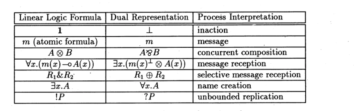
Figure 3 summarizes the connection between linear logic formula and process. Some of concurrent linear logic programming languages, including ACL and
Higher-Order ACL, are formalized using dual connectives. We show this dual representation in the second column (In the second column, positive and negative atoms are also exchanged).
A.3
Higher-Order
ACL
Higher-Order$\mathrm{A}\mathrm{C}\mathrm{L}[5]$ is based on Girard’ssecond-order linear$\mathrm{l}\mathrm{o}\mathrm{g}\mathrm{i}\mathrm{c}[1]$ with $\lambda$-abstraction.
Notethat withhigher-order linear logic, a predicate can take predicates as arguments,
Linear Logic Formula Dual Representation Process Interpretation
Figure 3: Connection between formula and process
can be also over predicates, hence processes can communicateprocesses and
commu-nication channels via a message.
Higher-Order ACL is equipped with an $\mathrm{M}\mathrm{L}- \mathrm{S}\mathrm{t}\mathrm{y}\mathrm{i}_{\mathrm{e}}$ type system. Note that types
in Higher-Order ACL have nothing to do with Curry-Howard isomorphism, because
we regard formulas as processes, not as types. Higher-Order ACL took the similar
approach to$\lambda \mathrm{p}\mathrm{r}\mathrm{o}\log$ in introducing types. We have a special type$‘ \mathit{0}$’ for propositions.
Computationally, it corresponds to the type of processes and messages. $intarrow \mathit{0}$ is a
type of predicate on integers. Computatinally, it is a type of processes or messages
which take an integer as an argument. $(intarrow \mathit{0})arrow \mathit{0}$ is a type of processes or
messages which take a process or a message that takes an integer as an argument.
$(intarrow \mathit{0})arrow int$ is a type of functions which take a process that takes an integer as
an argument, and returns an integer. Processes can bedefined and used
polymorphi-cally, by using let proc $\mathrm{p}(\mathrm{x})=$ el in e2 end statement, which is analogous fun
statement in$\mathrm{M}\mathrm{L}$. Process definitions could be expressed by a formula $!(p(X)-\mathrm{o}e1)$, (or
$!(p(x)0-e1)$ by the dual encoding), which corresponds to clause in traditional logic
programming. However, we prefered to interpret itas let$p=\mathrm{f}\mathrm{i}\mathrm{x}(\lambda p.\lambda X.e1)$
in
$e2$endwhere fix is a fixpoint operator, for the introduction of $\mathrm{M}\mathrm{L}$-style polymorphic type
system. It makes sense, because unlike traditionallogic programming, we can restrict