ヘルムホルツ共鳴器列を取り付けたトンネル内を伝播する音響孤立波
阪大
基礎工
杉本信正
(Nobumasa SUGIMOTO)
Abstract
Itis demonstrated theoretically that anacousticsolitarywave canbepropagated
in atunnel with a periodic array of Helmholtz resonators, ifthe dissipative
ef-fectsaremadenegligiblysmall. Aswave propagation in suchaperiodic system is
known asthe Bloch waves, the array can giverise tothe dispersion necessaryto
formation ofthe solitary wave. Explicit profiles of the solitarywaves are shown
by solving the steady-wave solutions to the nonlinear wave equations derived
previously. It is found that the solitarywave is compressive and that it is
propa-gated with aspeedslower than the usual soundspeed $a_{0}$, i.e. subsonic, but faster
than $a_{0}(1-\kappa/2)$ inthe linear long-wavelimit, $\kappa$being asmall parameter
repre-senting the ratio of the cavity’s volume tothe tunnel’svolume per axial spacing
between the neighboring resonators. As the propagation speed approaches the
upper bound, the height of the solitary wave increases to approach the limiting
height, while as the speed approaches the lower bound, the solitary wave tends
to be the soliton solution of the Korteweg-de Vries equation. It is also found
that whilenosolutionsexist for thespeedbelow thelowerbound, the shockwave
may be propagated for the speed above the upper bound, i.e. supersonic, but
accompanyingnonlinearly oscillatory wavetrain downstream.
1. Introduction
It has long beenbelieved that an acoustic $\mathrm{s}\mathrm{o}\mathrm{l}\mathrm{i}\mathrm{t}\mathrm{o}\mathrm{n}^{\uparrow}$
cannot exist in the pure air. For the
airitself is not adispersive materialbutrather adissipative
one.
Ofcourse, the dispersionoccurs geometrically but it is too strong to balance with the weak nonlinearity for the
soliton to be generated.
But itwasrecently revealedtheoretically thatthesoliton ispossible
even
inthe acousticwaves
propagating ina
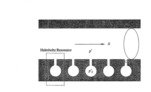
tunnel, ifa suitable array of Helmholtz resonators (called simplyresonators hereafter) is connected as shown in Fig.1 [1]. This
was
discovered in thecourse
of the investigations to inhibit emergence of the acoustic shockwave
generated bytravelling ofahigh-speed train ina tunnel [2]. In thefurther study, itwas shown that for
the acoustic solitonto be generated, the array oftheresonators
can
be generalized totheperiodic array ofany side branches as far as they are closed and acoustically compact [3,
4].
Wave propagation in suchaperiodicsystemmaybe termedthe acousticBloch
waves
[5,6] by analogy with that in the quantum mechanics [7]. The spatial periodicity gives rise
to the dispersion even in the mode of plane
waves.
For nonlinear acoustic Bloch waves,the Korteweg-de Vries (K-dV) equation can be derived commonly under the continuum
Figure 1. A tunnel with a periodic arrayof Helmholtz resonators.
approximation for distribution of the side branches $[3,4]$. This approximation holds
sub-stantially when a wavelength is much longer than the axial spacing between the
neigh-boring side branches.
In view of these results, this paper abandons the assumption for the K-dV equation to
be derived and investigates under what conditions a solitary wave is possible in steady
propagation of nonlinear acoustic waves in the tunnel with the array of resonators. By
neglecting all dissipative effects, we examine steady-wave solutions to the nonlinear wave
equations derived previously [1]. It is noted that these equations still exploit the
contin-uum approximation. The conditions for the steady-wave solutions to exist are clarified
and their explicit profiles are displayed.
2. Governing equations
At the outset, we present the governing equations derived for the one-dimensional
propagation of nonlinear acoustic waves in the tunnel with the array of resonators. If
the dissipative effects due to the wall friction and the diffusivity of sound are negligibly
small, they
are
given in the dimensionless form as follows (see (2.28) and (2.29) in $[1]\ddagger$):$\frac{\partial f}{\partial X}-f\frac{\partial f}{\partial\theta}=-K\frac{\partial g}{\partial\theta}$ , (2.1)
$\frac{\partial^{2}g}{\partial\theta^{2}}+\Omega g=\Omega f$, (2.2)
with$f=f(X, \theta)$ and$g=g(X, \theta)$wherethedefinitionsof the symbolsarebrieflydescribed
in the following (see also Fig.1).
Denoting the small order of nonlinearity by $\epsilon(<<1),$ $\epsilon f$ and $\epsilon g(f\sim g\sim O(1))$
denote the
excess
pressure $p’$ and $p_{2}’$over
the atmospheric $p_{0}$ in the tunnel and in thecavity of the resonator, respectively, normalized in reference to $p_{0}$ as $[(\gamma+1)/2\gamma]p’/p_{0}$
and $[(\gamma+1)/2\gamma]p_{2}’/p_{0}$ where $\gamma$ stands for the ratio of the specific heats and the factor
$(\gamma+1)/2\gamma$ is introduced for convenience. Letting the dimensional coordinate along the
tunnel be $x$ and the time be $t,$ $X$ and $\theta$ denote,
respectively, the far-field coordinate
$\epsilon\omega x/a_{0}$ and the retarded time $\omega(t-x/a_{0})$ in a frame moving with the usuallinear
sound
speed $a_{0}$, where $\omega$ is a typical angular frequency. The parameters $K$ and $\Omega$
measure
theratio of the smallness ofthe resonator to the nonlinearity and the ratio of the resonator’s
natural angular frequency$\omega_{0}$ to $\omega$, defined, respectively, as follows:
$K= \frac{\kappa}{2\epsilon}$ and $\Omega=(\frac{\omega_{0}}{\omega})^{2}$
,
(2.3)where $\kappa(\ll 1)$ is the ratio of the cavity’s volume relative to the tunnel’s volume per axial
spacing between the neighboring resonators. These parameters may be removed from
(2.1) and (2.2) by the replacement
$(f, g)arrow(Kf, Kg)$ and (X,$\theta$) $arrow(X/K^{\sqrt{\Omega},\sqrt{\Omega}}\theta/)$ . (2.4)
In the following, therefore, $K$ and $\Omega$ are set equal to unity without loss of generality.
3. Propagation of solitary
waves
In search of a solitary wave, we examine steady-wave solutions to (2.1) and (2.2),
assuming $f$ and$g$dependon$X$ and $\theta$ only through a combination
$\theta-sX(\equiv\zeta),$ $s$ beinga
constant. The inverse of$s$gives the propagation velocity in the (X,$\theta$) space. But weshall
see
to what $s$ corresponds in the original $(x, t)$ space. Taking account of the replacement(2.4) and the definition of $\Omega,$ $\zeta$ is written as
$\zeta=\omega_{0}[t-(1+\epsilon KS)_{X}/a_{0}]=\omega_{0}\{t-X/[a_{0}(1-\epsilon K_{S})]+O(K\epsilon)^{2}\}$. (3.1)
Hence we findthat $a_{0}(1-\epsilon Ks)$ corresponds to the original propagation velocity. Because
$\epsilon Ks$ is small enough, the propagation is directed toward the positive
$x$ axis irrespective
of the sign of$s$
.
Rewriting (2.1) and (2.2) in terms of$\zeta$, it follows that
$-s \frac{\mathrm{d}f}{\mathrm{d}\zeta}-f\frac{\mathrm{d}f}{\mathrm{d}\zeta}=-\frac{\mathrm{d}g}{\mathrm{d}\zeta}$ , (3.2)
$\frac{\mathrm{d}^{2}g}{\mathrm{d}\zeta^{2}}+g=f$
.
(3.3)For the solitary wave, we
assume
the undisturbed state far ahead as $xarrow\infty$ with $t$fixed. Thus the boundary conditions are imposed as follows:
Using these conditions, (3.2) is immediately integrated to give the first integral:
$g= \frac{1}{2}f^{2}+sf$
.
(3.5)Next multiplying (3.3) by $\mathrm{d}g/\mathrm{d}\zeta$ and writing $f\mathrm{d}g/\mathrm{d}\zeta$
as
$f(f+s)\mathrm{d}f/\mathrm{d}\zeta$ by (3.5), (3.3)is integrated with respect to $\zeta$ where $\mathrm{d}g/\mathrm{d}\zeta$is assumed to vanish as $\zetaarrow-\infty$, as inferred
by (3.4). Further eliminating $g$ by virtue of (3.5), it thenfollows that
$( \frac{\mathrm{d}f}{\mathrm{d}\zeta})^{2}=\frac{f^{2}(f_{+}-f)(f-f_{-})}{4(f+S)^{2}}$, (3.6)
with
$(f_{+}-f)(f-f_{-})=-f2-4(s- \frac{2}{3})f-4s(s-1)$
,
(3.7)and
$f_{\pm}=-2(s- \frac{2}{3})\pm\sqrt{-\frac{4}{3}s+\frac{16}{9}}$ , (3.8)
where the sign is vertically ordered. In passing, itcan be confirmedby (3.6) that $\mathrm{d}f/\mathrm{d}\zetaarrow$
$0$ as $farrow \mathrm{O}$ so that $\mathrm{d}g/\mathrm{d}\zetaarrow \mathrm{O}$ as $\zetaarrow-\infty$
.
In (3.6), areal solution $f$exists only when the right-hand side is non-negative. For it to
bebounded, $f_{\pm}$ must be realso that $s\leq 4/3$. Then the solution is possible in theinterval
$f_{-}\leq f\leq f_{+}$. Figure 2 shows the graph of $f_{\pm}$ as the functions of $s$. For $1<s<4/3$
or
$s<0,$ $f_{\pm}$
are
both negative orboth positive. If so, the point $f=0$ is not included in theinterval $f_{-}\leq f\leq f_{+}$ and there cannot exist continuous solutions$\mathrm{s}\mathrm{a}\mathrm{t}\mathrm{i}\mathrm{S}y_{\mathrm{i}}\mathrm{n}\mathrm{g}$the boundary
conditions (3.4). Therefore such a case should be excluded. For
$0<s<1$
, two typesof the solutions
are
possible in the intervals $0\leq f\leq f_{+}$or
$f_{-}\leq f\leq 0$, separately. Inthe latter interval, however, $\mathrm{d}f/\mathrm{d}\zeta$ diverges as $farrow-S$ because $f_{-}$ is always less $\mathrm{t}\mathrm{h}\mathrm{a}\mathrm{n}-s$
for
$0<s<1$
(see Fig.2). The divergence implies that the legitimacy of (2.1) and (2.2)is lost since the dissipative terms in the original equations, especially the second-order
derivative with$\beta$ remain nolongersmall in the vicinity of the divergent point. Therefore
we discard the solution in the interval $f_{-}\leq f\leq 0$
.
In the interval $0\leq f\leq f_{+},$ $(3.6)$ is immediately led to the quadrature:
$\int_{f}^{f}+\frac{2(f’+s)}{f’\sqrt{(f_{+}-f’)(f-f_{-})}},\mathrm{d}f’=\pm\zeta$. (3.9)
Thisintegral is straightforwardly executed to yield
$4 \tan^{-1}\sqrt{\frac{f_{+}-f}{f-f_{-}}}-\frac{2s}{\sqrt{-f_{+}f_{-}}}\log|\frac{[\sqrt{-f_{-}(f_{+}-f)}-\sqrt{f_{+}(f-f_{-})}]^{2}}{(f_{+}-f_{-})f}|=\pm\zeta$, (3.10)
Figure 2. Graph of$f_{\pm}$ versus $s$.
Figure$3(\mathrm{a})$ depictsthe explicit profilesof$f$in $\zeta$for thevalues of$s$from0.2 to 0.8by the
step 0.2, while Fig.$3(\mathrm{b})$ depicts the profiles of
$g$ corresponding to those in Fig.$3(\mathrm{a})$. As $f$
tends to vanish, it is found from (3.10) that $\zeta$ approaches both infinity so that $f$ can also
$\mathrm{s}\mathrm{a}\mathrm{t}\mathrm{i}_{\mathrm{S}}\mathrm{f}_{Y}$the undisturbed boundary conditions
downstream as $\zetaarrow\infty$. Hence the solution
(3.10) representsthe solitary wave symmetric with respect to $\zeta=0$. As $s$ becomes small,
the height of the solitary wave $f_{+}$ increases to approach the limiting value 8/3. Exactly
for $s=0$, however, (3.10) ceases to be valid because $f_{-}$ vanishes (while $f_{+}=8/3$). Then
$f$ represents no longer the solitary wave but a sinusoidal wavetrain given by
$f= \frac{8}{3}\cos^{2}(\frac{\zeta}{4})$ (3.11)
This is also available by taking the limit of (3.10) as $sarrow \mathrm{O}$. Then the first term on the
left-hand side gives (3.11), whereas the second term drops out. It should be remarked
that (3.11) cannot $\mathrm{s}\mathrm{a}\mathrm{t}\mathrm{i}\mathrm{s}\mathrm{f}_{Y}$ the boundary condition (3.4).
Hence the height of the solitary
waves is less than 8/3.
As $s$ approaches unity, on the other hand, $f_{+}$ tends to vanish. In this limit, the
prop-agation velocity in (3.1) approaches $a_{0}(1-\epsilon K)=a_{0}(1-\kappa/2)$, which corresponds to the
speed in the linear long-wave limit, though exactly given by $a_{0}/(1+\kappa)^{\frac{1}{2}}$ from the Bloch
dispersion relation (see (64) in the reference [6]). Let $s$ be $1-\alpha/3$ where $\alpha(0<\alpha<<1)$
measures
the closeness to unity. In terms of $\alpha,$ $f_{+}$ and $f_{-}$ are given, respectively, by $\alpha+O(\alpha^{2})\mathrm{a}\mathrm{n}\mathrm{d}-4/3+O(\alpha)$ to the lowest order. Then (3.10) is approximatedto be $f=\alpha \mathrm{s}\mathrm{e}\mathrm{c}\mathrm{h}2\sqrt{\frac{\alpha}{12}}\zeta$ , (3.12)
with$\zeta=\theta-X+\alpha x/3$. This is nothing but the soliton solution to the K-dVequation [1]. Hence it is found that the soliton solution is included among the solitary-wave solutions
(b)
$g$
$\zeta$ $\zeta$
Figure 3. (a): Profiles of$f$ for the solitary waves with $K=1$ where the solid, dotted, broken
and chain lines represent, respectively, the profiles in the cases with $s=0.2,0.4,0.6$ and 0.8.
(b): Profiles of$g$ calculated by (3.5) for the solitarywaves corresponding to those of$f$ in (a).
4. Propagation of shock waves
So far, we have assumed
$0<s<1$
. Let us examine solutions for$1<s<4/3$
or$s<0$. Obviously, then, there cannot exist continuoussolutions satisfying (3.4). But (3.2)
and (3.3) allow a discontinuous solution as a weak solution. Let the discontinuity in $f$
be located at $\zeta=0$. In the vicinity of it, assume $f$ be expressed approximately in the
form$f=f_{1}h(\zeta)$ where $h(\zeta)$ denotes the unit step function and $f_{1}$ isan arbitrary constant
representing the magnitude of discontinuity. Integration of (3.2)
over
a narrow regionacross $\zeta=0$ from $\zeta=0-\mathrm{t}\mathrm{o}\zeta=0+\mathrm{y}\mathrm{i}\mathrm{e}\mathrm{l}\mathrm{d}\mathrm{s}$
$[sf+ \frac{1}{2}f2-g]_{\zeta=0_{-}}^{\zeta=}0+=0$ , (4.1)
where the square bracket $[\ldots]_{\zeta=0_{-}}^{\zeta}=0+\mathrm{s}\mathrm{i}\mathrm{g}\mathrm{n}\mathrm{i}\mathrm{f}\mathrm{i}\mathrm{e}\mathrm{S}$ a change of a quantity across $\zeta=0$. In
consisitent with the step in $f,$ $(3.3)$ requires that
$[g]_{\zeta=0_{-}}^{\zeta}=0+=[ \frac{\mathrm{d}g}{\mathrm{d}\zeta}]_{\zeta=}^{\zeta=0+}0-0=$ . (4.2)
While$g$ and$\mathrm{d}g/\mathrm{d}\zeta$must be continuous across$\zeta=0$ due to the ‘inertia’ of the resonator,
the magnitude of discontinuity $f_{1}$ is found to be given by $-2s$. Although $f_{1}$ may be
arbitrary taken, it is known in the theory of gas dynamics that only the compressive
shock wave $(f_{1}>0)$ is admissible. This prohibits taking a positive value of$s$. For $s=0$,
the discontinuity in $f$ disappears but the higher-order derivative of $f$ may be subjected
ofthe origin, while $f$ is taken to vanish for $\zeta<0$. Then the second-order derivative of$f$
jumps
across
$\zeta=0$.Allowingthe discontinuity at $\zeta=0$ in solutions, we nowsolve (3.2) and (3.3) for $\zeta>0$
.
Ofcourse, $f$ and$g$ are identically
zero
for $\zeta<0$. The boundary conditions at $\zeta=0+\mathrm{a}\mathrm{r}\mathrm{e}$taken as follows:
$f–f_{1}=-2s$ and $g= \frac{\mathrm{d}g}{\mathrm{d}\zeta}=0$ at $\zeta=0+$ (4.3)
Integration of (3.2) leads to the same first integral as (3.5). Making use ofthis and (4.3),
(3.3) is integrated, after multiplied by $\mathrm{d}g/\mathrm{d}\zeta$, to yield
$( \frac{\mathrm{d}f}{\mathrm{d}\zeta})^{2}=\frac{(f-f_{1})}{4(f+S)^{2}}F(f;s)$ , (4.4)
with
$F(f;s)=-f3-(2s- \frac{8}{3})f^{2}-\frac{4}{3}Sf+\frac{8}{3}s2$ (4.5)
In orderto integrate (4.4), the roots of the cubicequation$F(f;s)=0$must bespecified.
Examining the first-order derivative of $F$ with respect to $f$, it is found that $F$ has two
extrema for $s<0$, one in $f<0$ and the other in $f>0$, and that both extremal values of
$F$
are
positive. In fact, letting the extremum be located at $f=f_{e}$,we
have$F(f_{e};s)=- \frac{2}{3}(s-\frac{11}{9})fe+\frac{8}{3}2(s-\frac{f_{\mathrm{e}}}{6})^{2}>0$ , (4.6)
where $f_{e}$ satisfies $-3f_{e}^{2}-2(2_{S}-8/3)f_{e}-4s/3=0$. The above facts indicate that the
cubic equation has one positive root $f_{2}$ and two complex conjugate roots. Furthermore
$f_{2}$ is found to be greater than $f_{1}$ and the limiting height 8/3 because
$F(f_{1;}S)=16s^{2}>0$
,
$F( \frac{8}{3};s)=\frac{8}{3}s^{2}-\frac{160}{9}s>0$.
(4.7)As
$-S$ increases, $f_{2}$ also increases unlimitedly as well as $f_{1}$ but the difference $f_{2}-f_{1}$approaches the value 4. This is found from the asymptotic expression of$f_{2}$ givenby
$f_{2}=-2s+4+ \frac{4}{s}+O(S^{-2})$, as $sarrow-\infty$
.
(4.8)Hence the solution to (4.4) with (4.5) is possible for $f_{1}\leq f\leq f_{2}$. Equation (4.4) is
then reduced to the integral:
The algebraic integrand can also be expressed in terms ofthe Jacobian elliptic function
by introducing the following auxiliary variable $z$ defined by (see the formulae 259.07 in
[8], pp.134-135)
$f’= \frac{c_{1}f_{2}(1-\mathrm{c}\mathrm{n}z)/+C_{2}f_{1}(1+\mathrm{C}\mathrm{n}z’)}{c_{1}(1-\mathrm{c}\mathrm{n}z)\prime+C2(1+\mathrm{c}\mathrm{n}z)},$ , (4.10)
and
$\mathrm{c}\mathrm{n}z=\frac{-c_{2}(f-f_{1})+c1(f2^{-}f)}{c_{2}(f-f_{1})+c1(f2^{-}f)}$ , (4.11)
where
cn
$z$ stands for the Jacobi’s elliptic function $\mathrm{c}\mathrm{n}(Z, k)$ withthe modulus $k$ given by$k^{2}= \frac{(f_{1^{-}}f2)^{2}-(c1-C2)^{2}}{4c_{12}c}$ , (4.12)
and $c_{1}$ and $c_{2}$
are
defined by$c_{1}^{2}=H(f_{1})=f_{1}^{2}+cf_{1}+ \frac{8s^{2}}{3f_{2}}$ , (4.13)
$c_{2}^{2}=H(f_{2})=f2^{+}C2f_{2}+ \frac{8s^{2}}{3f_{2}}$ , (4.14)
where $H(f;\mathit{8})=F(f;s)/(f_{2}-f)=f^{2}+cf+8s^{2}/3f_{2}$ with $c=f_{2}+2s-8/3$. It then
follows $\mathrm{h}\mathrm{o}\mathrm{m}(4.9)$ that
$\pm(\zeta-\zeta 0)=\frac{2}{\sqrt{c_{1}c_{2}}}\int_{z}2K(k)[\frac{c_{2}f_{1}+c1f_{2}+(c_{2}f_{1}-c\mathrm{l}f_{2})\mathrm{c}\mathrm{n}Z\prime}{c_{1}+c_{2}-(c_{1}-C2)\mathrm{c}\mathrm{n}z},+s]\mathrm{d}z’$ (4.15)
where $K(k)$ denotes the complete elliptic integral of the first kind, which should not be
confused with $K$ in (2.1) and $\zeta_{0}$ is chosen so that $f$ may take $f_{1}$ at $\zeta=0$
.
This gives the form of the nonlinearly oscillatory wavetrain behind the shock
wave.
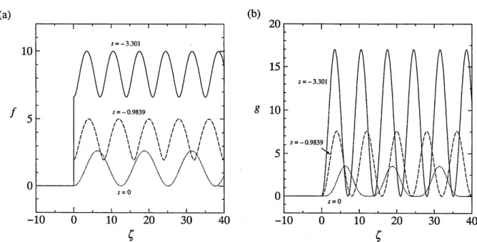
Upon integrating (4.15) numerically, Figure $4(\mathrm{a})$ depicts the profiles of $f$ for the shock
waves
followed by the wavetrain where the solid and broken lines represent, respectively,the profiles in the cases with $f_{2}=10$ ($f_{1}\approx$ 6.603 and $s\approx$ -3.301) and $f_{2}=5(f_{1}\approx$
1.968 and $s\approx-0.9839$), while the dotted line represents the sinusoidal wavetrain (3.11)
for $s=0$
.
Figure$4(\mathrm{b})$ depicts the profiles of$g$ corresponding to those in Fig.$4(\mathrm{a})$.5. Results and discussions
Here we summarize the results of the analysis in the preceding sections. It is found
that the steady propagation into the undisturbed state far ahead is classified, depending
on
the propagation velocity $s$, into two classes, one being the class ofthe solitarywaves
for $0<s<1$ and the other that of the shockwaves for $s<0$. For $s\geq 1$, no steady-wave
oth-(b)
$g$
$g$ $g$
Figure 4. (a): Profiles of $f$ for the shock waves with $K=1$ where the solid and broken lines
represent, respectively, the profiles in the cases with $f_{2}=10$ ($f_{1}\approx 6.603$ and $s\approx-3.301$) and
$f_{2}=5$ ($f_{1}\approx$ 1.968 and $s\approx$ -0.9839), while the dotted lines represent (3.11) for $s=0$. (b):
Profiles of$g$ calculated by (3.5) for the shockwavescorresponding to those of$f$ in (a).
er values of $K$, the excess pressure $\epsilon f$ and $\epsilon g$ for the given profiles become large in
proportion to $K$. On the other hand, the propagation velocity in the $(x, t)$ space is
retarded from the sound speed $a_{0}$ by the amount $\epsilon Ks$ proportional to $K$ where note that
$\epsilon Ks$ is equivalent to $\kappa s/2$ by the defintion of $K$ in (2.3). Hence while the shock waves
are obviously supersonic, it is found that the solitary waves are subsonicbut the speed is
faster than $a_{0}(1-\kappa/2)$.
As $s$ decreases from unity, the height of the solitary wave increases monotonously (see
Fig.3) while it is propagated faster. For $s$ slightly below unity, the solitary wave is well
approximated by the soliton solution of the K-dV equation. The deviation from unity
determines the height of the soliton. As $s$tends to vanishfrom above, the height increases
but it must be less than the limiting value 8/3 in the dimensionless form. This limiting
height corresponds to the excess pressure $p_{l}’$ given by
$\frac{p_{l}’}{p_{0}}=\frac{8\gamma}{3(\gamma+1)}\kappa$ . (5.1)
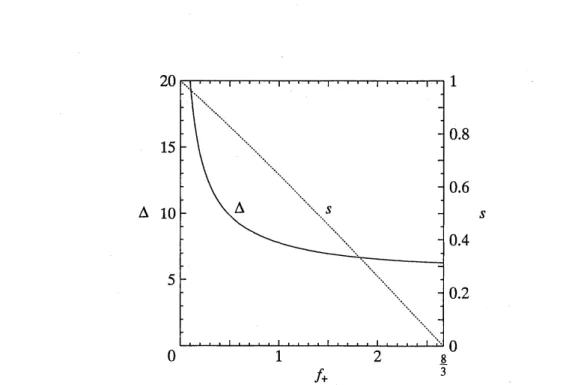
As the solitary wave becomes higher, it is seen in Fig.3 that its width is reduced. One
common check in identifying experimentally the solitary wave is to plot the half width
against the maximum height. The half width $\triangle$ is defined as
$2|\zeta(f_{+}/2)|$ when $\zeta$ in (3.10)
is regardedas the function of$f$. Figure 5 shows therelation between $f_{+}$ and $\triangle$ where the
Figure 5. Relation between the maximum height of the solitarywave $f_{+}$ and its half width $\Delta$
where the dotted lines show the relation between $f_{+}$ and $s$ given by (3.8).
the limiting height 8/3, $\triangle$ approaches $2\pi$, while as $f_{+}$tends tovanish, $\triangle$becomes inversely
proportional to the square root of the height $f_{+}(=\alpha)$ (see (3.12)).
As was shown in [1], it is the case with $\Omega>>1$ that the K-dV equation is derived
asymptotically so that the soliton is possible. Let us see the connections between this
approximation and the present results. Provided a typical frequency $\omega$ for the solitary
waveisdefinedas$\pi/D,$ $D$beingatemporalhalf width in$t$, inotherwords, $D$ is regardedas
ahalfperiod of the sinusoidalwave of frequency $\omega$, then $\Omega$ in (2.3) is given by $(\omega_{0}D/\pi)^{2}$.
Since $\omega_{0}D$ corresponds to $\triangle$ in
$\zeta,$ $\Omega[=(\triangle/\pi)^{2}]$ is found to be greater than 4 for the
limiting height. Hence it is found that the solitary wave exists for $\Omega>4$ in the present
definition.
For anegativevalue of$s$, the shockwave appears with nonlinearly oscillatory wavetrain
downstream and it propagates faster than the soundspeed $a_{0}$. The greater the magnitude
of discontinuity becomes, the faster it propagates. But the wavetrain tends to be a
sinusoidal one with the $\mathrm{p}\mathrm{e}\mathrm{a}\mathrm{k}-\mathrm{t}\mathrm{o}-\mathrm{P}^{\mathrm{e}}\mathrm{a}\mathrm{k}$amplitude 4 and withperiod $2\pi$ in $\zeta$. This is found
by noting that as $-Sarrow\infty$, we have the relations that $f_{1}\approx f_{2}arrow-2s,$ $c_{1}\approx c_{2}\approx-2s$
and $k^{2}arrow 0$ so that $\pm(\zeta-\zeta_{0})$ in (4.15) takes the value $\pi-z$ with $\cos\zeta_{0}=-1$ and $\mathrm{c}\mathrm{n}z$
is reduced to $\cos\zeta$. On the other hand, when the discontinuity vanishes for $s=0$, the
wavetrain is given by the sinusoidal one (3.11) with the $\mathrm{P}\mathrm{e}\mathrm{a}\mathrm{k}- \mathrm{t}_{0}$ peak amplitude 8/3 and
withperiod$4\pi$ in $\zeta$. Interms ofthe frequency in$t$, the wavetrain for $s=0$ oscillates with
the halfof the resonator’s natural frequency, while $\mathrm{a}\mathrm{s}-sarrow\infty$, it tends to oscillate with
the natural frequency. For the intermediate values of $s$, it is observed in Fig.4 that the
6. Conclusion
This paper has investigated the steady propagation ofnonlinear acoustic
waves
in thetunnel with the arrayofHelmholtz resonators. It has been revealedthat the compressive
solitary wave is possible and its speed is subsonic but faster than $a_{0}(1-\kappa/2)$, depending
on the parameter $\kappa$ for the smallness of the resonator. As mentioned in Introduction,
the acoustic soliton is predicted universally in propagation along
a
long duct with aperiodic array of side branches. But it should be noted that the solitary wave obtained
here depends crucially on the specific type of the side branchs, i.e. the response of the
Helmholtzresonator in thepresentcontext. Therefore if other sidebranchesareconnected,
solitary waves different in shape would be obtained.
Besidesthe solitary waves, it is found that thesupersonicshockwaveis alsopossiblefor
thespeedfasterthan$a_{0}$. But since the long-wave approximationbreaksdown at the shock
front, it is evident that the validity of the solutions is lost in the exactsense. Yet it is worth
emphasizing that the resonators
are
dormant in response to the discontinuous change inpassage ofthe shock front and the long-wave approximation is still fully satisfied for the
wavetrain. Ifwetake account of
a
small effect due to thediffusivityof sound (representedby the second-order derivative with the small parameter$\beta$ inthe originalequation (2.28)$)$,
the discontinuity is diffused to be replaced by
a
rapid but continuous transition layer.References
1. Sugimoto, N. 1992 Propagation of nonlinear acoustic waves in atunnel with an array of
Helmholtz resonators. J. Fluid Mech. 244, pp.55-78.
2. Sugimoto, N. 1993 ‘Shock-free tunnel’ for future high-speed trains. in Proceedings
of
International
conference
on speed-up technologyfor
railway and maglev vehicles, (JapanSociety of Mechanical Engineers, Tokyo) Vol.2, pp.284-292.
3. Sugimoto, N. 1993 Ongeneration of acoustic soliton. In $AdvanCe\mathit{8}$ inNonlinear$A_{CouS}tic\mathit{8}$
(ed. H. Hobaek) pp.545-560. World Scientific.
4. Sugimoto, N. 1995The generationofanacoustic solition andsolitontube. Proc. Estonian
Academy
of
Sciences Physics $\xi y$ Mathematics 44, 1, pp.56-72.5. Bradley, C. E. 1991 AcousticBlochwave propagation in aperiodic waveguide. Technical
Report
of
Applied$Re\mathit{8}earch$ Laboratories, ARL-TR-91-19 (July) (The UniversityofTexasat Austin).
6. Sugimoto, N.
&Horioka,
T. 1995 Dispersion characteristics of sound waves in a tunnelwith an array ofHelmholtz resonators. J. Acoust. Soc. Am. 97, pp.1446-1459.
7. Kittel, C. 1976 Introduction to solid state physics. (John Wiley&Sons, New York, 5th
edition).
8. Byrd, P. F.