Stable ROW-Type Weak Scheme for Stochastic Differential Equations(2nd Workshop on Stochastic Numerics)

Stable

ROW-Type

Weak Scheme for

Stochastic Differential

Equations

小守良雄 (Yoshio Komori) 三井斌友 (Taketomo Mitsui)

Department of Information Engineering

Graduate School

of Human In

ormatics

School

of

Engineering,

Nagoya University

Nagoya

University

Abstract

A stable weak scheme of ROW-type is proposed forstochastic differentialequation so asto

reserve itsstability in the mean squaresense and to be of order 2. Desirable restrictionsof

nu-mericalscheme are investigated to deriveaspecified one. Throughsome numerical experiments

for thescheme, thestability property and theconvergence order are verified.

1

Introduction

Numerical methodisone of effective means toobtain the informationabout stochasticphenomena

which analytically unsolvable stochastic differential equations (SDEs) present. Among such

meth-ods weak schemes are often used to get approximations ofsample characteristics of solutions of

SDEs. So far many weak methods have been proposed in the literature (forexample, [3, 9, 10]).

On the other hand the importance of stability consideration on numerical schemes for SDEs

has been acknowledged similarly as in the case ofordinary differential equations (ODEs) toavoid

explosion of numerical solution. Several concepts of analytical stability for SDEs are considered

([1, 5]), while more numerical stability concepts are treated due to many different test equations

with additive or multiplicative noise ([6, 8]).

However for SDEs with multiplicative noise we can find a very few weak schemes which have

the stability property corresspondingto $A$-stability in ODEs ([2, 8]). Therefore the followings are

our goal of the features of anew scheme proposed in the presentpaper.

1) The scheme is ROW-type of weak order 2.

2) For homogeneous $d$-dimensional linearSDEs with the diffusion coefficient matrix having only

real eigenvalues,

i) the scheme is asymptotically stable in the mean-square sense with any step-size if the

underlying SDEs are asymptoticallystable, and

ii) exactly reserves the instability with sufficiently small step-size if the underlying SDEs

are not stable.

3) The scheme is $A$-stableas for ODEs if the diffusion coefficient matrix vanishes.

We will give numericalexperiments for the scheme and show that the scheme worksvery well with

2

Preliminaries

In this section we will introduce some notations and concepts forlater use.

Suppose that

$dz(t)= \sum_{j=0}^{p}g^{j}(t, Z(t))dw(jt)$, $z(t_{0})=z_{0}$ (fixed), $t\geq t_{0}$, (2.1)

is a $d$-dimensional SDE which has a unique solution. The sense of the stochastic differential will

be specified later. Here $dw^{0}(t)\equiv dt$ and $w^{j}(j=1, \ldots,p)$ stand for mutually independent Wiener

processes. Furthermore we assume $g^{j}(j=0,1, \ldots,p)$ are continuous with _{respect to}$t$, and satisfy

$g^{j}(t, 0)=0$ for all $t\geq t_{0}$,

so that $z(t)\equiv 0$ is the solution of (2.1) with initial value _{$z_{0}=0$}

.

We will call this trivial solution

as the equilibrium position. In the sequel we generally assume $z(t)\in C^{d}$ for convenience’ sake.

Thefollowing concepts can be found in [1].

Definition 2.1 ($\mathrm{m}.\mathrm{s}$

.

stability, $\mathrm{a}.\mathrm{m}.\mathrm{s}$

.

stability) The equilibrium position is said to be stable

in the mean-square sense ($m.s$

.

stable, in short) if,

for

every$\epsilon>0$, there exists a $\delta>0$ such that

$\sup$ $E[||Z(t)||2]\leq\epsilon$ for $||z_{0}||\leq\delta$,

$t_{0}\leq t<\infty$

where $||z(t)||$ stands

for

the norm $(z(t)^{*}Z(t))^{1/}2$ (the mark * means the conjugate $tmns\mu_{S}i\iota i_{\mathit{0}}n$).

Further

_if

$\lim_{tarrow\infty}E[||z(t)||^{2}]=0$ for all$z_{0}$ in a neighborhood of $0,$’

the equilibrium positionis said to be asymptotically stable in the mean-square sense ($a.m.s$

.

stable).

When $E[||z(t)||^{2}]$ is replaced by $||E[z(t)Z(t)^{*}]||=( \sum_{i,j=1}^{d}|(E[z(t)z(t)^{*}])ij|2)^{1}/2$ in Definition

2.1, the (asymptotical) stabilityin the mean-square sense turns to the (asymptotical) stability of

the second moment $E[z(t)_{Z(}t)^{*}]$

.

Let $c_{P(C,c)}^{\iota d}$ be the totality of $l$ times continuously differentiable_$C$-valued functionson $C^{d}$,

all of whose partial derivatives of order less than or equalto $l$ have polynomial growth. Let _$N$ be a

natural number, and for an end time $T>0$, set the step-size $\Delta t=(T-t\mathrm{o})/N$ and the step-point

$t_{n}=t_{0}+n\Delta t(n=0,1, \ldots, N)$

.

Denote by $z(t_{n})$ and $z_{n}$ the exact and approximate solution of

SDE, respectively, at time $t_{n}$

.

Definition 2.2 (weak order) $([\mathit{1}\mathit{0}\mathit{1})$A time discrete approximation _{$Z_{N}$} issaid to converge weakly

with order $q$ at time $t_{N}$ as $\Delta tarrow \mathrm{O}$

if for

each $G\in C_{P}^{2(q+1)}(Cd, c)$ there exists a positive constant

$C$ independent

of

$\Delta t$ and satisfying

$|E[G(Z(t_{N})]-E[G(zN)]|=C\Delta t^{q}$

.

We will restrict ourselves with autonomous SDEs with $p=1$ and omit the superscripts with

It\^o-type,the following explicit Runge-Kutta scheme proposed by PLATEN (p.485 in [10]) is known.

$z_{n+1}$ $=$ $z_{n}+ \frac{1}{2}(g^{0}(_{\hat{Z}}n)+g(0)zn)\Delta t$

$+ \frac{1}{4}(g^{1}(Z_{n})++g(1z-)n+2g^{1}(zn))\Delta w_{n}$

$+ \frac{1}{4}(g^{1}(z_{n})+-g^{1}(z^{-})n)\{(\Delta w_{n})2-\Delta t\}\Delta t^{-}\frac{1}{2}$, (2.2)

$\hat{z}_{n}$ $=$ $z_{n}+g^{0}(zn)\triangle t+g^{1}(Zn)\Delta w_{n}$,

$z^{\pm}$

$=$ $z_{n}+g^{0_{(Z_{n})\Delta}1}t\pm g(Zn)^{\sqrt{\Delta t}}$

.

Here, $\Delta w_{n}$, which stands for the difference $w(t_{n+1})-w(t_{n})$, is realized by the pseudo-random

number whose expectation and covariance are $0$ and $\Delta t$, respectively. This schemeis proved to be

ofweak order 2.

The numerical counterpart of the a.m.s. concept is given in [2]. as follows.

Definition 2.3 (a.m.s. stability for numerical scheme) A numerical scheme is saidtobe

asymp-toticallystable in the mean-square sense ($a.m.s$

.

stable) with a step-size $\Delta t$

if

the numerical scheme

appliedto the$SDE$, in which the equilibriumposition is a.$m.s$

.

stable,

satisfies

thefollowingequation

for

the step-size.

$\lim_{narrow\infty}E[||Z_{n}||^{2}]=0$

.

3

Test

equations

for numerical stability

We will introduce a linear $d$-dimensional system of SDEs and a linear scalar SDE both with

mul-tiplicative noise. These equations devoted to stability analysis have the common necessary and

.sufficient

condition for the a.m.s. stability oftheir equilibrium positions.

Consider the following homogeneous linearIt\^o-type SDEs in $R^{d}$

$dx(t)=Ax(t)dt+Bx(t)dw(t)$, $x(t_{0})=x_{0}$ (fixed $R^{d}$-value), _{$t\geq t_{0}$}, (3.1)

provided that $d\cross d$real matrices $A$ and $B$ are simultaneously diagonalizable. The second moment

$P(t)=E[x(t)x^{\tau}(t)]$ _{of the solutionsatisfies} the equation ([1])

$\frac{dP}{dt}(t)=AP(t)+P(t)A^{T}+BP(t)B^{\tau}$, P$(t_{0})$

- $-=$.

$x_{0^{X_{0}}}.-.T$

.

(3.2)

The above assumption implies the diagonalizing matrix$T$ togive the identities

$\Lambda=T^{-1}AT$, $\Gamma=T^{-1}BT$,

where $\Lambda$ and $\Gamma$ stand for the diagonal matrices

$A=$

,

$\Gamma=$

,

and these diagonal components $\lambda_{i}(A)$ or $\lambda_{i}(B)(i=1, \ldots,d)$ denote eigenvalues of$A$ or $B$,

Let$x(t)=Tz(t)$

.

Notethat $x(t)\in R^{d}$, but $z(t)\in C^{d},$$T\in C^{d\mathrm{x}d}$

.

Putting_{$Q(t)=E[z(t)_{Z^{*}(}t)]$},

we have

$P(t)=TQ(t)\tau*$

.

(3.3)

Substitution of(3.3) into (3.2) and simplificationyield

$\frac{dQ}{dt}(t)=\Lambda Q(t)+Q(t)\Lambda^{*}+\Gamma Q(t)\tau*$, $Q(t_{0})=(T^{-1_{X_{0}}})(T^{-}1x\mathrm{o})^{*}$

.

Specifying the componentsof$Q(t)$ by

$Q(t)=$

,

we can get

$\frac{dq_{||}}{dt}..(t)=(2\Re(\lambda|.(A))+|\lambda_{i}(B)|2)qii(t)$, $q_{ii}(t_{0})=((T^{-}1_{X_{0}})(T-1x_{0})*)_{i}:$

.

The relationships$||P(t)||\leq E[||x(t)||^{2}]$ and$E[||x(t)||^{2}]=\mathrm{t}\mathrm{r}\mathrm{a}\mathrm{C}\mathrm{e}P(t)$ show that the$\mathrm{m}.\mathrm{s}$

.

stability

is equivalenttothestability ofthe secondmoment ([1]). Itis easy to verify thatthe fact is alsotrue

in the complex case. That is,the stability of$q_{ii}(t)$ is equivalent to the stability of$Q(t)$

.

Therefore

from (3.3) the stability of$qii(t)$ is equivalent to the $\mathrm{m}.\mathrm{s}$

.

stability in (3.1). This equivalence also

holds for the a.m.s. stability.

Thus we can conclude that the a.m.s. stabilityof the equilibrium position of(3.1) is equivalent

to the following inequalities.

$2\Re(\lambda|(A))+|\lambda_{i}(B)|^{2}<0$, $(i=1, \ldots,d)$

.

(3.4)

Denote by$j$ the index for which _{$2 \Re(\lambda_{j}(A))+|\lambda_{j}(B)|^{2}=1\leq i\leq\max(2\Re(d\lambda_{i}(A))+|\lambda:(B)|^{2})$} holds, and

further introduce thenotations

$\tilde{\lambda}=\Re(\lambda_{j}(A))$ and $\tilde{\sigma}=\pm|\lambda_{j}(B)|$, (3.5)

which leads an equivalent condition

$2\tilde{\lambda}+\tilde{\sigma}^{2}<0$ (3.6)

of(3.4).

Assume that

$\lambda=\lambda_{j()}A$, $\sigma=\pm\lambda_{j}(B)$

.

The necessary and sufficient condition of the a.m.s. stability for the equilibrium position of scalar

It\^o-typeequation

$dz(t)=\lambda z(t)dt+\sigma z(t)dw(t)$, $z(t_{0})=z_{0}$, $z(t)\in C$

.

(3.7)

turns out tobe consistent with (3.6). Thereforethea.m.s. stability of(3.7)is equivalent tothat of

(3.1).

Equation (3.7)is interpreted to Stratonovich-type equation

$dz(t)=\hat{\lambda}z(t)dt+\sigma z(t)\mathrm{o}dw(t)$, $z(t_{0})=z_{0}$, $z(t)\in C$, (3.8)

where $\hat{\lambda}=\lambda-\frac{\sigma^{2}}{2}$

.

Then the condition (3.6) can be written in the form

$\Re(\hat{\lambda})+\{\Re(\sigma)\}^{2}<0$

.

(3.9)

4

Significance

of

a.m.s.

stability

in

numerical schemes

Applying Platen’s scheme (2.2) to Eq. (3.7), weobtain

$z_{n+1}= \{1+\lambda\Delta t+\sigma\Delta wn+\lambda\sigma\Delta t\Delta w_{n}+\frac{1}{2}\sigma\{2\Delta w_{n}^{2}-\Delta t\}+\frac{1}{2}\lambda^{2}\Delta t^{2}\}zn$

.

Define the amplification factor as

$P( \Delta t, \Delta w_{n})\equiv 1+\lambda\triangle t+\sigma\Delta w_{n}+\lambda\sigma\Delta t\Delta w_{n}+\frac{1}{2}\sigma^{2}\{\Delta w_{n}^{2}-\Delta t\}+\frac{1}{2}\lambda^{2}\Delta t^{2}$

.

(4.1)

The expectation of the squared $P(\Delta t, \Delta w_{n})$ is given by

$E[|P( \Delta t,\Delta wn)|^{2}]=1+(2\tilde{\lambda}+\tilde{\sigma}^{2})\Delta t+2(\tilde{\lambda}+\frac{1}{2}\tilde{\sigma}^{2})^{2}\Delta t^{2}|\lambda|^{2}(\tilde{\lambda}+\tilde{\sigma}^{2})\Delta t^{3}+\frac{1}{4}|\lambda|^{4}\Delta t^{4}$

.

Therefore, the necessary and sufficient condition fora.m.s. stability of scheme (2.2)is given by

$(2 \tilde{\lambda}+\tilde{\sigma}^{2})\Delta t+2(\tilde{\lambda}+\frac{1}{2}\tilde{\sigma}^{2})2\triangle t^{2}+|\lambda|^{2}(\tilde{\lambda}+\tilde{\sigma}^{2})\Delta t^{3}+\frac{1}{4}|\lambda|4\Delta t^{4}<0$

.

Here introduction of notations $X=\tilde{\lambda}\Delta t,$ $\mathrm{Y}=\infty s(\lambda_{j}(A))\Delta t$and $W=\tilde{\sigma}^{2}\Delta t$ yields

$2X+W+2(X+ \frac{1}{2}W)^{2}+(X^{2}+\mathrm{Y}^{2})(X+W)+\frac{1}{4}(X^{2}+\mathrm{Y}^{2})^{2}<0$

.

(4.2)

Denotethe left-hand side term by $MS_{p}(X,\mathrm{Y},W)$

.

On theother hand the necessary and sufficient

condition,in which the equilibrium position of(3.7) is a.m.s. stable, can be expressed with

$2X+W<0$

.

(4.3)

Thismeans that under the restriction of(4.3),the triplet (X,$\mathrm{Y},$$W$)satisfying(4.2)gives the a.m.s.

stability criterion ofthe scheme (2.2) when it is appliedto the test equation (3.7).

Second, we will consider the stability with respect to expectation. From (4.1), we have

$E[P( \Delta t, \Delta wn)]=1+\lambda\Delta t+\frac{1}{2}\lambda^{2}\Delta t^{2}$

.

Therefore the condition, in which the expectation $E[z_{n}]$ converges to$0$ as $narrow\infty$, is

$|1+ \lambda\Delta t+\frac{1}{2}\lambda^{2}\Delta t^{2}|<1$

.

We will call it the stability in expectation ($\mathrm{e}$

.

stability, in short). Define

$E_{p}(X,Y) \equiv|1+(X+\mathrm{i}\mathrm{Y})+\frac{1}{2}(X+\mathrm{i}\mathrm{Y})^{2}|$,

then the necessary and sufficient condition, in which the expectation $E[z(t)]$ of the solution of (3.7)

converges $0$ as$tarrow\infty$, can be expressed with $\tilde{\lambda}<0$, which impies

$X<0$

.

Under these circumstances, we will show numerically that the a.m.s. stability is significant.

The 2-dimensional equation

serves the numerical test. The parameters are specified as $\alpha=3,$ $\beta=-100,$ $\gamma=-25,$ $x_{1}(t_{0})=1$, $x_{2}(t_{0})=0$

.

Calculationshows

$X= \frac{\gamma+\sqrt{\gamma^{2}+4\beta}}{2}\Delta t=-5\Delta t$, $\mathrm{Y}=0$, $W=\alpha^{2}\Delta t=9\Delta t$

.

Since

$2X+W=-\Delta t<0$,

the equilibrium position of(4.4)is a.m.s. stable.

The region of$\mathrm{e}$

.

stability $\{(X,Y);E(pX,Y)<1\}$ is shown as the shadowed zone in Fig. 4.1.

In the Figure points on the $X$-axis correspond to those for $\Delta t=2^{-6},2^{-5},$

$\ldots,$

$2^{-1}$, respectively, in

the order closer to the origin. The evaluated $MS_{p}(X,\mathrm{Y}, W)$ arelisted in Table 4.1 for every $\Delta t$

.

$\mathrm{Y}$

Figure 4.1: The region of$E_{p}<1$

Table 4.1: Arithmetic means and second moments at $T=5$ byscheme (2.2)

Since the two points corresponding to $\Delta t=2^{-3}$ and $2^{-2}$ on Fig. 4.1 satisfy the condition

$E_{p}(X,\mathrm{Y})<1$,onemightexpect that the arithmeticmean $\langle$$x_{N})$ oftheir numerical solutions is close

to $0$ as $N$ becomes large. Nevertheless, it explodes numerically as observed in Table 4.1. This

the existence of the paths that are far from$0$

.

In such a case the arithmetic mean can hardly be close

to $0$ because the computer simulationshave only a finite number of the paths. Consequently even

if one wants to know only arithmetic means, one cannot ignore the $\mathrm{m}.\mathrm{s}$

.

stability. This example

suggests the significance of a.m.s. stabilityin numerical schemes.

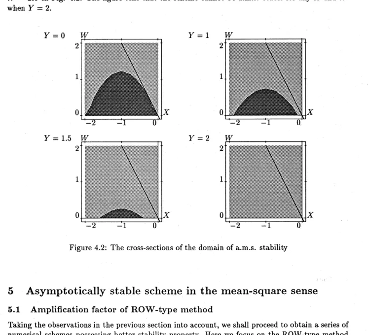
Finallywe note that the set $\{(X,Y, W)\}$ satisfying $MS_{p}(X,\mathrm{Y}, W)$ becomes to a domain in the

$3-\dim$ space, which can be called the domain ofa.m.s. stability. We show in Fig. 4.2 the

cross-sections of the domain of the scheme (2.2) with several planesof$\mathrm{Y}=\mathrm{c}\mathrm{o}\mathrm{n}\mathrm{s}\mathrm{t}$

.

Theregion satisfying

$2X+W<0$ and $W\geq 0$ means (3.7) is a.m.s. stable. The region is the part below the straght line

$W=2X$ in Fig. 4.2. The figure tells that the scheme cannot be a.m.s. stable for any $X$ and $W$

when $Y=2$

.

$\mathrm{Y}=0$ $\mathrm{Y}=1$

$Y=2$

Figure 4.2: The cross-sections of the domain ofa.m.s. stability

5

Asymptotically stable scheme

in

the

mean-square

sense

5.1

Amplification

factor of ROW-type method

Taking the observations in the previous section intoaccount, we shall proceed toobtain aseries of

of$m$ stages ([12]) given by

$\mathrm{Y}_{1}$. _$=$ $[I-\gamma\Delta w_{n}0_{\frac{\partial g^{0}}{\partial z}}(z_{n})]-1$

$\cross[\sum_{j=0}^{1}a^{j}i\Delta w^{j}gnj(Zn+\sum_{l=1}^{i-1}\alpha_{i}l\mathrm{Y}_{l})+\sum_{\iota}^{-}i=11\{_{i=0}\sum^{1}\gamma i\iota w\Delta j\frac{\partial g^{j}}{\partial z}jn(Z_{n})\mathrm{Y}_{l}\}]$, (5.1)

$z_{n+1}$ $=$ $z_{n}+ \sum_{j=1}^{m}c_{jj}\mathrm{Y}$

for SDE (2.1)interpreted in the Stratonovich sense. Here $\Delta w_{n}^{0}\equiv\Delta t$

.

Consider the scalar linear Stratonovich-type SDE

$dz(t)= \sum_{j=0}^{1}\hat{f}^{j}Z(t)\mathrm{o}du^{\dot{p}}(t)$, $z(t_{0})=z_{0}$

.

(5.2)

Applicaton of(5.1) to (5.2) implies the stage values as

$\mathrm{Y}_{i}=\sum_{=j0}^{1}\Delta w_{n}j\hat{f}j[a_{i}Zjn+\sum l=1i\mu_{\iota}^{j}\dot{.}\mathrm{Y}_{l}]$, (5.3)

where

$\mu_{il}^{j}=\{$

$a_{ii}^{jj}\alpha_{i\iota}+\gamma il$ $(i>l)$,

$\gamma$ $(i=l, j=0)$ ,

$0$ $(i=l, j=1)$

.

Hence introducing the notations

$\mathrm{Y}=[Y_{1},\mathrm{Y}_{2}, \ldots,Y_{m}]^{T}$, $a^{j}=[a_{1’ 2}^{jj\ldots T}aa^{j}]$, _{$c=[c1,c2, \ldots,cm]T$}

and

$U_{j}=$

, we obtain

$\mathrm{Y}=\sum_{j=0}^{1}\Delta w\hat{f}^{j}jn[aZn+U_{i^{\mathrm{Y}}}]j$, (5.4)

$-c^{T}\mathrm{Y}+z_{n}+1=z_{n}$

.

(5.5)

Composition of(5.4) and (5.5) yields

$[I- \sum_{0j=-c}^{1}\Delta\phi\hat{f}nU_{j}\tau j$

Calculationby Cramer’s ruleleads to theidentify

$\det[I-\sum_{j=0}^{1}\Delta_{1\dot{d}}\hat{f}njU_{j}+\sum_{j=0}^{1}\Delta\tau\dot{d}_{n}\hat{f}^{j}aC]jT$

$z_{n+1}=$

$\det[I-\sum_{0j=}^{1}\triangle w^{j}n\hat{f}jU_{j]}$

$z_{n}$

.

Put $\Delta W_{j}=\hat{f}^{j}\Delta w_{n}^{j}$ and define the amplificationfactor as

$\det[I-\sum_{=j0}^{1}\Delta W_{ji}U+\sum_{j=0}^{1}\Delta W_{j}a\mathrm{c}jT]$

$R(\Delta W_{0}, \Delta W1)\equiv$

$\det[I-\sum_{0i=}\Delta WjUj]1$

In what follows, we restrict the method (5.1) in the case of$m=4$

.

Then the denominator of

$R(\Delta W_{0,1}\Delta W)$ is factorized as

$\det[I-\sum_{j=0}^{1}\Delta WjUj]=D^{4}$, (5.7)

where $D=1-\gamma\Delta W_{0}$

.

On the other hand, by calculation using the condition (Appendix $(\mathrm{A})$) in

which the method (5.1)is of weak order 2,the numerator becomes

$\det[I-\sum^{1}\triangle W_{j}U_{j}j=0+\sum_{j=0}^{1}\triangle Wjac]j\tau$

$=$ $D^{4}+(_{j=} \sum^{1}\Delta Wj)\mathrm{o}D^{3}+\{(\frac{1}{2}-\gamma)\Delta W_{0}^{2}+(1-\gamma)\Delta W0\Delta W_{1}+\frac{1}{2}\Delta W_{1}^{2\}D^{2}}$ (5.8)

$+ \{T_{3}0\Delta W0^{3}+T_{21}\Delta W_{0^{\Delta}}^{2}W_{1}+(\frac{1}{2}-\gamma)\Delta W0\Delta W^{2}1+\frac{1}{6}\Delta W_{1\}D}^{3}$

$+T_{40} \Delta W_{0}4+\tau_{31}\Delta W_{0^{\Delta W}1}3+T_{22}\Delta W_{0}^{22}\Delta W_{1}+T_{13}\Delta W_{0}\Delta W_{1}^{3}+\frac{1}{24}\Delta W_{1}^{4}$

.

Here $T_{1j}$ means a polynomial of the formula parameters.

5.2

Desired

restrictions

on

ROW-type method

We shall impose the following four conditions on the ROW-type method. (Refer back to the goal

listedin Introduction.)

Assuming that $\hat{f}^{1}=0$ and _{$\Delta W_{1}=0$} hold, weobtain

$R( \Delta W_{0},\mathrm{o})=1+\frac{1}{D}\Delta W_{0}+\frac{1}{D^{2}}(\frac{1}{2}-\gamma)\Delta W_{0}^{2}+\frac{1}{D^{3}}T_{3}0\Delta W0^{3}+\frac{1}{D^{4}}\tau_{40}\Delta W_{0}4$ (5.9)

from (5.7) and (5.8). If $\gamma>0,$ $R(\triangle W_{0}, \mathrm{o})$ is analytic for $\Re(\Delta W0)<0$

.

Since we assume the

necessary and sufficient condition for $A$-stability of the ODE-case is that for all $\Delta W_{0}$ satisfying

$\Re(\Delta W_{0})=0$ and any $\gamma>0$ the inequality

$|R(\Delta W0,0)|2\leq 1$ _(5.10)

holds ([4]).

On the other hand, we can recognize that in the Fig. 4.2 the whole $X$-axis never be included

in the stability region. This means that Platen’s scheme is not $A$-stable in the ODE-case. In other

words, for $A$-stable methods in the ODE-case, the whole $X$-axis in the $X\mathrm{Y}W$-portrait should be

included in the domain ofa.m.s. stability. Therefore we impose A-stability in the ODE-caseas the

first restriction on the ROW-type method.

Assume _{a combination of the coefficients in the Stratonovich-type SDE} (5.2) as $\hat{f}^{0}=-\mathcal{E}$ and

$\hat{f}^{1}=\epsilon+\mathrm{i}\eta$ for _{$1\gg\epsilon>0$}

.

The equation turns out to

be a.m.s. stable because the condition (3.9)

is satisfied. As $\epsilonarrow 0$, we have

$R( \Delta W_{0}, \triangle W1)arrow 1-\frac{1}{2}(\eta\Delta w^{1})^{2}n+\frac{1}{24}(\eta\triangle w^{1})^{4}n+\{(\eta\triangle w^{1})n-\frac{1}{6}(\eta\Delta w_{n}^{1})^{3}\}$

from $\Delta W_{0}arrow 0$ and $\triangle W_{1}arrow \mathrm{i}\eta\Delta w_{n}^{1}$

.

This yields

$E[|R( \triangle W0, \triangle W_{1})|^{2}]arrow 1-\frac{5}{24}\eta^{6}\Delta t^{38}+\frac{35}{192}\eta\Delta t^{4}$

as $\epsilonarrow 0$

.

Therefore in this case the ROW-scheme (5.1) is impossible to be a.m.s. stable with

any $\Delta t$

.

As we have seen above, even if $\hat{f}^{0}\in R$, the ROW-schme (5.1) cannot be a.m.s. stable

with any $\Delta t$ provided $\hat{f}^{1}\in C$

.

Thus we restrict (3.8) in the case of $\hat{f}^{0}\in C$ and $\hat{f}^{1}\in R$, that is,

$\hat{f}^{0}=\lambda-\frac{\overline{\sigma}^{2}}{2}$ and $\hat{f}^{1}=\tilde{\sigma}$

.

(Recall the definition ofthe quantity $\tilde{\sigma}$ in (3.5).)

We can then represent $E[|R(\triangle W0, \Delta W1)|^{2}]$ as a function with arguments only$X,$ $Y$ and $W$

.

We will make the method (5.1) satisfying

$E[|R(\triangle W_{0}, \triangle W_{1})|^{2}]<1$ (5.11)

under $W\geq 0$andthecondition (4.3). Itmeans that (5.1)isnumerically a.m.s. stablewithany $\Delta t$

.

When $\gamma>0,$ $E[|R(\Delta W0, \Delta W1)|^{2}]$ is analytic in the left half-plane of X-W for any Y. Therefore

(5.11) holds if and only if(5.10) holds and the inequality

$E[|R(\Delta W_{0}, \Delta W_{1})|^{2}]\leq 1$

is satisfied on the extreme line $W=-2X$ ofthe condition (4.3). Our second restriction is for the

above inequality to hold.

The curve which representsthe relationship $E[|R(\triangle W_{0}, \Delta W_{1})|^{2}]=1$ in the$XW$-plane is the

boundary of the region of a.m.s. stabilityfor(5.1). We willmakethescheme(5.1) sothat the slope

ofthe boundary curve at the origin (X,$W$) $=(\mathrm{O}, 0)$ is equal to $-2$

.

This means that the stability

region of(5.1) is consistent with the analytic a.m.s. stability of (3.7) in the neighborhood of the

origin. This is our third restriction.

The last restriction is as follows. For $X=0$ and $W\neq 0$,

$E[|R(\Delta W_{\mathit{0}}, \Delta W1)|^{2}]>1$ (5.12)

is desirable because then SDE (3.7) is not stable.

We impose these four restrictions in addition to the conditions for weak order 2 on the

5.3 Specification formula parameters

By calculations we find

$|D\{^{2}|R(\triangle W_{0},\mathrm{o})|^{2}-|D|^{2}$ ($\leq 0$ for $\Re(\Delta W_{0})=0$),

which is derived from the left-hand side of(5.10), and

$|D|^{2}E[|R(\Delta W0,\Delta W1)|^{2}]-|D|^{2}$ ($>0$ for $X=\Re(\Delta W_{0})=0$), (5.13)

which is obtained from the left-hand side of (5.12), are polymomials of$\Delta t$ of degree 8 and their

leading coefficients coincide. Denote by $l_{c}$ the coefficient. For the condition (5.10), $l_{c}$ should be

non-positive. On the other hand, $l_{c}$ should be non-negative for the condition (5.12). Henceforth

we shall take that $l_{c}=0$ and the second leading coefficient of (5.13) is positive. Then, for large

enough $W,$ $(5.12)$ is satisfied.

Summing up ouranalyses,we will decide the parameters of the scheme (5.1)sothatit possesses

fourproperties describedabove andis of weak order2. Theorderconditions of(5.1)for weak order

2 can be derived according to an analysis previously described in [12] and is listed inAppendix A.

The selection $\gamma=\frac{1}{2}$ and $T_{30}=T_{40}=0$ suggested from the formulae (A.2), (A.3), (A.4) and

(A.5) reduces (5.9) into a simpleequation

$R( \Delta W_{0},0)=1+\frac{1}{D}\Delta W_{0}$,

which leads the equation

$|R( \triangle W_{0},\mathrm{o})|^{2}-1=|\frac{1}{D}|^{2}2X$

.

Therefore we can satisfy both (5.10) and $l_{c}=0$ when $\gamma=\frac{1}{2}$,because

$|R(\Delta W_{0}, \mathrm{o})|^{2}=1$ if$X=0$

.

A set of the formulaparameter satisfying all of the desired conditions is listed in Appendix B.

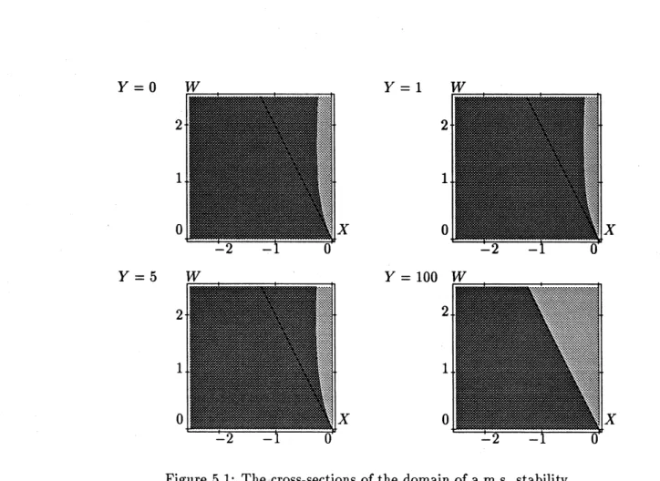
We call the scheme (5.1) with these parameters by Scheme A. Fig. 5.1 shows the cross-sections

$Y=0$ $\mathrm{Y}=1$

$\mathrm{Y}=5$

Figure 5.1: The cross-sections of the domain of a.m.s. stability

6

Numerical

tests

for the

new

scheme

Solution of the test equation (4.4) with the parameters $\alpha=3,\beta=-100$ and $\gamma=-25$ by Scheme

A is listed in Tab. 6.1, which clearly shows that the expectations as well as the mean squares are

solved stably.

Table 6.1: Arithmetic means and second moments by Scheme A

Next wewill show anumerical experimentin an oscillatory SDE case. Assume that the

param-eters $\alpha=0.5,$ $\beta=-37$ and $\gamma=-2$ in the equation (4.4),which imply

$dx(t)=x(t)dt+x(t)dw(t)$

, $x(t_{0})=$

.

(6.1)

The eigenvalues of the drift coefficient $\mathrm{a}\mathrm{r}\mathrm{e}-1\pm \mathrm{i}6$, which yield the inequality

Thus the equilibrium position of(6.1)is a.m.s. stable.

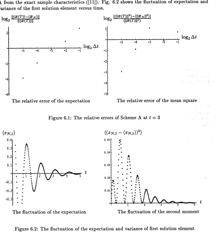
We showin Fig. 6.1 the tendency of the numerical error of Scheme A versus step-size. Herethe

numerical erroris taken as its relative value of the approximate sample characteristicsby Scheme

A from the exact sample characteristics ([11]). Fig. 6.2 shows the fluctuation of expectation and

variance of the first solution element versus time.

$\perp’ \mathrm{h}\mathrm{e}\mathrm{r}\mathrm{e}\iota \mathrm{a}\mathrm{t}\mathrm{l}\mathrm{v}\mathrm{e}$ error$\mathrm{o}l$ theexpectation The relatlve error$\mathrm{o}l$ themean square

Figure6.1: The relativeerrors ofScheme A at $t=3$

$(x_{N.1})$ $((x_{N1}--(x_{N.1}))2)$

The fluctuation ofthe expectation The fluctuation of the second moment

Figure 6.2: The fluctuation of the expectation and variance of first solution element

7

Concluding remarks

Through the discussion about the numerical stability for SDEs, we raised for numerical schemes

several conditions (ref. tothem listed in Introduction), which wererealized with Scheme A of an

However,someproblemsare remained unsolved. First,thereare still cases in which the variance

of the solution of an SDE must diverge theoretically, but converges numericaly. Thisphenomenon

could be found, for example, when $\alpha=3,$ $\beta=-1/4$ and $\gamma=-3$in the test equation (4.4)

intro-duced in the paper. This combination ofparameters impliesthat the equation is a.m.s. unstable.

Trajectory tracing of the analytical solution with pseudo-random numbers on computer, however,

shows convergence. Henceforth the sameoccurs in the numerical simulation with Scheme A for the

equation, too. The reason may be considered that the pseudo-Wiener process does not have paths

ofbig magnitude at the end point of time. The phenomenon suggests that the instability ofthe

numerical scheme may be influenced by pseudo-random numbers. Thus we need to take enough

care of the instability of the original SDE even if the numerical result is stable.

Second, we need further study when an eigenvalue of the matrix of diffusion coefficient is a

complex number. In the case when the imaginary part vanishes in the stochastic part ofthe test

equation (3.7),itwas shownthat Scheme A was a.m.s. stable with any$\Delta t$if(3.7)was a.m.s. stable

(ref. to 5 in the present paper).

However in thecaseof the complexnumberin the stochastic part ofit,thesituation is different.

To confirm it, putting $X=\Re(\lambda)\triangle t$ and $\mathrm{Y}=\infty s\lambda\Delta t$ as Section 4, denoting by $U=\{\Re(\sigma)\}^{2}\Delta t$ and

$V=\{\propto s(\sigma)\}2\Delta t$, we readily see that the condition (4.3) ofa.m.s. stability for (3.7) turns out to

$X<- \frac{1}{2}U^{2}-\frac{1}{2}V^{2}$

.

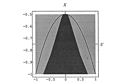
We have then fourquantities$X,\mathrm{Y},$$U$ and $V$tocontrolstability. For$\mathrm{Y}=0$and$V=1$, forinstance,

the region of Scheme A in $XU$-plane where the condition (5.11) is satisfied is shown in Fig. 7.1

(the shadowed region). The region does not

cover

the analytical stability region of (3.7) that is

below the parabola.

$X$

Figure 7.1: The stability region of Scheme A for$\mathrm{Y}=0$ and $V=1$

HOFMANN and PLATEN [7] try to investigate a way to overcome a similar problem to it, but

the schemes they handle with are restricted in lower order weak ones. Refer to [13], too. Therefore

Appendix

A

The order conditions

for

weak order

2

Here we introduce the following notations:

$A_{ij}$ $=$ $a_{i}\alpha_{ij}+\gamma_{i}0j$

’ $B_{ijj}=b_{i\alpha_{1}}\cdot+\gamma_{ij}1$, $A_{i}$ $=$ $\sum_{j=1}^{i-1}ajA_{i}j$, $B_{i}= \sum_{j=}^{\dot{|}}-11b_{j1j}B\cdot$, $\overline{B}_{i}$ _$=$ $\sum_{j=1}^{i-1}b_{j}\alpha_{ij}$

.

$b_{1}c_{1}+b2c2+b3C3+b_{4}C_{4}$ $=$ 1

$a_{1}c_{1}+a_{2}c2+a_{3}C3+a4C4$ $=$ 1

$B_{2^{C_{2}+}}B_{3}C_{3}+B_{4}C_{4}$ $=$ $\frac{1}{2}$

$a_{1}B_{212}C+(a1B31+a_{2}B_{32})c_{3}+(a1B41+a2B42+a3B_{43})c_{4}$ $=$ $\frac{1}{2}$

$A_{21}b_{1}C_{2}+(A_{31}b_{1}+A_{32}b_{2})c_{3}+(A_{41}b_{1}+A_{42}b_{2}+A_{43}b_{3})c_{4}$ $=$ $\frac{1}{2}-\gamma$ (A.1) $A_{2}c_{2}+A_{3}c_{3}+A_{4}c_{4}$ $=$ $\frac{1}{2}-\gamma$ (A.2) $\overline{B}_{2}^{2}b_{2}C_{2}+\overline{B}_{3}^{2}b_{3}C_{3}+\overline{B}_{4}^{2}b_{4}c_{4}$ $=$ $\frac{1}{3}$

$a_{1}\overline{B}_{2}\alpha_{21}b_{2}c_{2}+\overline{B}_{3}(a1\alpha_{31}+a2\alpha 32)b_{33}c+\overline{B}4(a_{1}\alpha 41+a_{2}\alpha_{4}2+a3\alpha 43)b_{4^{C}4}$ $=$ $\frac{1}{4}$

$\alpha_{21}^{2}a_{2}b21c_{2}+a3(\alpha 31b_{1}+\alpha 32b_{2})2_{C_{3}+()}a_{4}\alpha 41b_{1}+\alpha_{42}b2+\alpha_{4}3b_{3}2_{C_{4}}$ $=$ $\frac{1}{2}$

$B_{2}B_{32}C_{3}+(B_{2}B_{42}+B3B43)c_{4}$ $=$ $\frac{1}{6}$

$A_{21}b_{1}B_{32}C_{3}+(A_{32}b2B_{43}+b_{1}(A_{21}B_{42}+A_{31}B_{43}))c4$ $=$ $- \frac{\gamma}{2}$ (A.3)

$a_{1}B_{21}B32c_{3}+(a_{2}B_{32}B_{43}+a_{1}(B_{21}B_{42}+B_{31}B_{43}))c4$ $=$ $\frac{1}{4}$

$A_{32}b_{1}B_{2}1c_{3}+(b_{1}(A_{42}B_{21}+A_{43}B_{31})+A_{43}b_{2}B_{3}2)C4$ $=$ $\frac{1}{4}-\frac{\gamma}{2}$ (A.4)

$\overline{B}_{2}^{3}b_{2}C_{2}+\overline{B}_{3}^{3}b_{3}C_{3}+\overline{B}_{4}^{3}b_{4}C_{4}$ $=$ $\frac{1}{4}$

$\overline{B}_{3}\alpha_{32}B_{2}b_{3}C_{3}+\overline{B}_{4}(\alpha 42B_{2}+\alpha 43B3)b4C4$ $=$ $\frac{1}{8}$

$B_{2}B32B43C_{4}$ $=$ $\frac{1}{24}$

$\overline{B}_{2}^{2}b2B32c3+(\overline{B}_{2}^{2}b_{242}B+\overline{B}_{34}^{2}b_{3}B3)_{C_{4}}$ $=$ $\frac{1}{12}$

$\mathrm{B}$

The

parameter

set

of

Scheme

A

$a_{1}$ $=$ $-1+\sqrt{3}$, $a_{2}=7- \frac{5\sqrt{3}}{2}$, $a_{3}= \frac{11}{2}-\frac{5\sqrt{3}}{2}$, $a_{4}= \frac{4}{3}-\frac{1}{\sqrt{3}}$,

$b_{1}$ $=$ 1, $b_{2}= \frac{1}{2}$ $b_{3}= \frac{1}{2}$ $b_{4}=1$,

$c_{1}$ $=$

$\frac{1}{6}$ $c_{2}= \frac{4(-7+4\sqrt{3})}{27}$, $c_{3}= \frac{37-16\sqrt{3}}{27}$, _{$c_{4}= \frac{2}{3}$}

$\alpha_{21}$ $=$ 1, $\alpha_{31}=\frac{1979+112(3^{\frac{3}{2}})}{1202}$, $\alpha_{32}=-\frac{777}{601}-\frac{112(3^{\frac{3}{2}})}{601}$,

$\alpha_{41}$ $=$ $- \frac{1}{4}$, _{$\alpha_{42}=1$}, $\alpha_{43}=\frac{1}{2}$ $\gamma=\frac{1}{2}$,

$\gamma_{21}^{0}$

$=$ $\frac{-29+11\sqrt{3}}{8}$, $\gamma_{31}^{0}=\frac{-20335+6199\sqrt{3}}{2404}$, $\gamma_{32}^{0}=\frac{21(167-3^{\frac{5}{2}})}{1202}$,

$\gamma_{41}^{0}$ _$=$ $\frac{70-37\sqrt{3}}{6}$, $\gamma_{42}^{0}=\frac{-4+\sqrt{3}}{3}$, $\gamma_{43}^{0}=\frac{-4+\sqrt{3}}{6}$

.

$\gamma_{21}^{1}$

$=$ $\frac{1}{4}$ $\gamma_{31}^{1}=\frac{73-112(3^{\frac{5}{2}})}{7212}$, $\gamma_{32}^{1}=\frac{3533+112(3^{\frac{5}{2}})}{3606}$ $\gamma_{41}^{1}$ _$=$ $\frac{71}{216}+\frac{2}{3^{\frac{5}{2}}}$, $\gamma_{42}^{1}=\frac{-91+16\sqrt{3}}{54}$, $\gamma_{43}^{1}=-\frac{1}{4}$

References

[1] L. Arnold. Stochastic

_Differential

Equations: Theory and Applications. John Wiley&Sons,

New York, 1974.

[2] S.S. Artem’ev. Thestabilityof numerical methods for solving stochastic differentialequations.

Bulletin

_of

the Novosibirsk Computing Center, 2, 1993.

[3] T.A. Averina and S.S. Artem’ev. A new family of numerical methods for solving stochastic

differential equations. Soviet Math. Dokl.,33:736-738, 1986.

[4] E. Hairer and G. Wanner. Solving Ordinary

_Differential

Equations II,

_Stiff

and

Differential-Algebraic Systems. Springer-Verlag, Berlin, 1991.

[5] R.Z. Has’minskii. Stochastic Stability

_{of Differential}

Equations. Sijthoff&Noordhoff

Interna-tional Publishers B.V., Netherlands, 1980.

[6] D.B. Hernandez andR. Spigler. Convergenceand stability ofimplicitrunge-kutta method for

systems with multiplicativenoise. BIT, 33:654-669, 1993.

[7] N. Hofmann and E. Platen. Stability ofsuperimplicitnumerical methods for stochastic

differ-ential equations. Technical Report SRR 015-94, The Australian National University, 1994.

[8] N. Hofmann and E. Platen. Stability of weak numerical schemes for stochastic differential

[9] J.R. Klauder and W.P. Petersen. Numerical integration of multiplicative-noise stochastic

dif-ferential equations. SIAM J. Numer. Anal., 22:1153-1166, 1985.

[10] P.E. Kloeden and E. Platen. Numerical Solution

of

Stochastic

Differential

Equations.

Springer-Verlag, Berlin, 1992.

[11] Y. Komori,Y. Saito,and T. Mitsui. Some issue in discrete approximate solution for stochastic

differential equations. Computers Math. Applic., 28:269-278, 1994.

[12] Y. Komori, H. Sugiura, and T. Mitsui. Rooted tree analysis of the order conditions of

ROW-type scheme for stochastic differential equations. Submitted.

[13] G.N. Milstein,E.Platen,and H. Schurz. Balanced implicit methods for stiff stochasticsystems.